
Using DBpedia to Enhance your Data in GraphDB
Following my article on Transforming Tabular Data into Linked Data using OntoRefine in GraphDB, the founder of Ontotext (Atanas Kiryakov) suggested I write a further tutorial using GraphDB for data reconciliation.
In this tutorial we will begin with a .csv of car manufacturers and enhance this with DBpedia. This .csv can be downloaded from here if you want to follow along.
Contents
Setting Up
Constructing the Graph
Reconciling your Data
Exploring the New Graph
Conclusion
Setting Up
First things first, we need to load our tabular data into OntoRefine in GraphDB. Head to the import tab, select “Tabular (OntoRefine)” and upload cars.csv if you are following along.
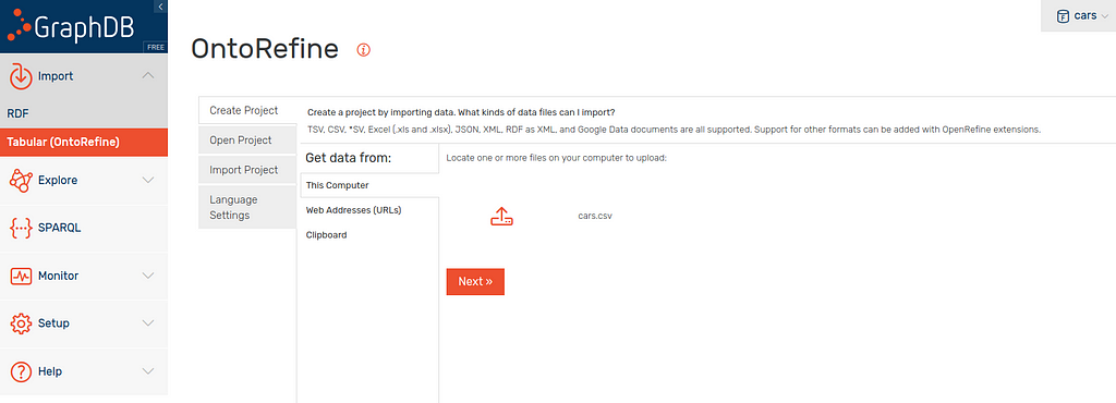
Click “Next” to start creating the project.
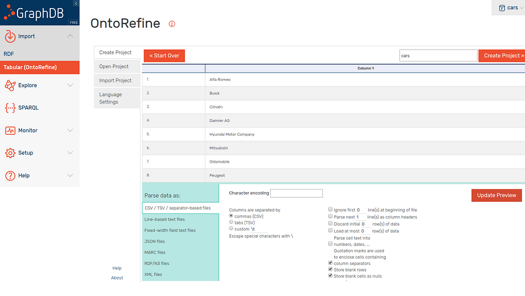
On this screen you need to untick “Parse next 1 line(s) as column headers” as this .csv does not have a header row. Rename the project in the top right corner and click “Create Project”.
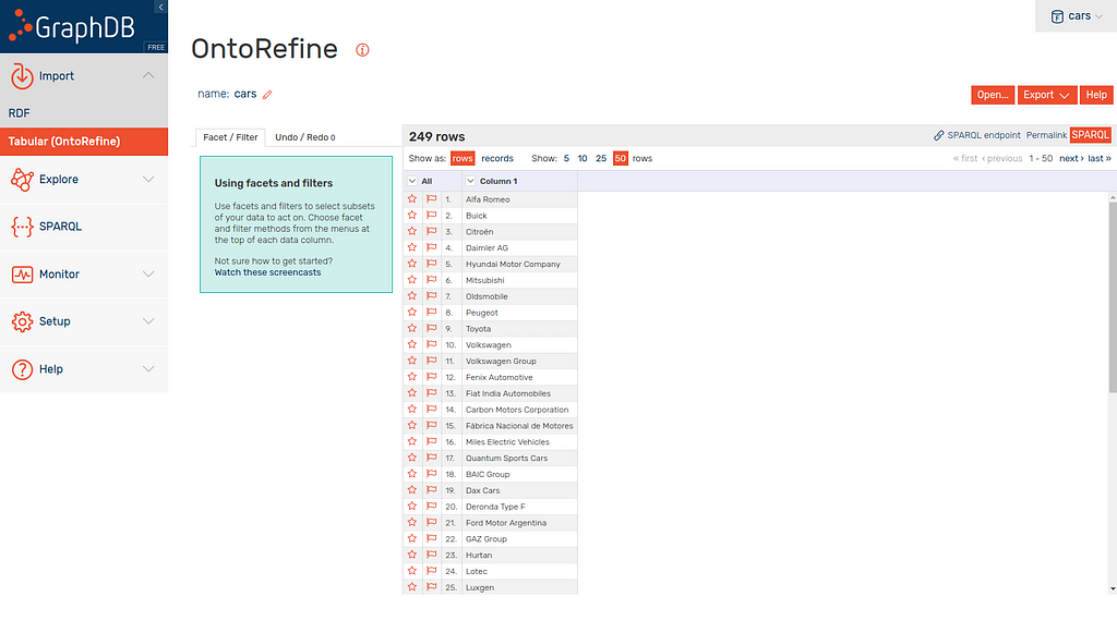
You should now have this screen (above) showing one column of car manufacturer names. The column has a space in it which is annoying when running SPARQL queries across so lets rename it.
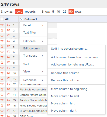
Click the little arrow next to “Column 1”, open “Edit Column” and then click “Rename this Column”. I called it “carNames” and will use this in the queries below so remember if you name it something different.
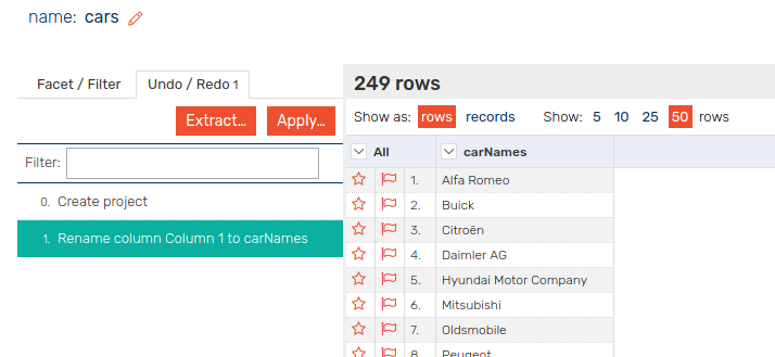
If you ever make a mistake, remember there is and undo/redo tab.
Constructing the Graph
In the top right of the interface there is an orange button titled “SPARQL”. Click this to open the SPARQL interface from which you can query your tabular data.
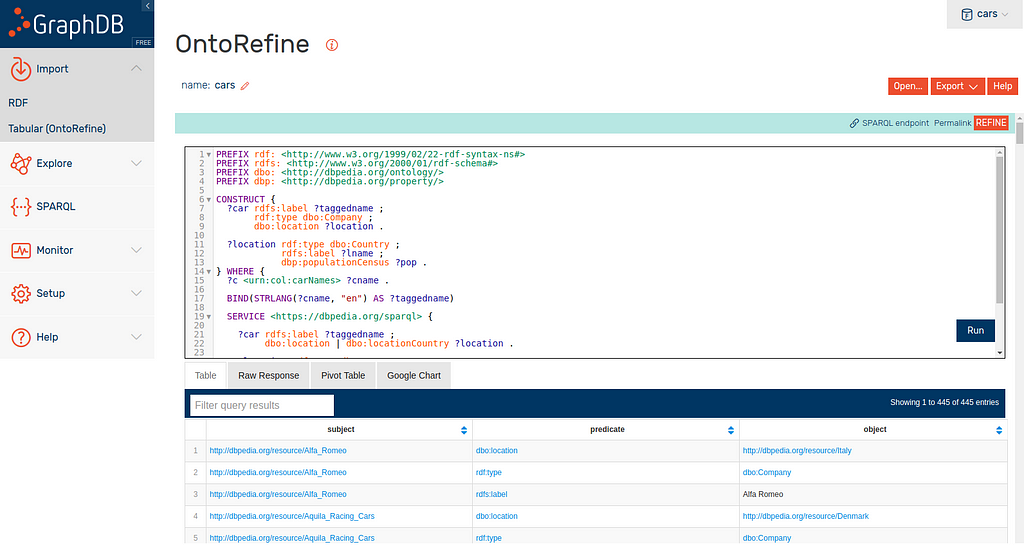
In the above screenshot I have run the query we want. I have have pasted it here so you can see it all and I go through it in detail below.
I use a CONSTRUCT query here. If you are new to SPARQL entirely then I recommend reading my tutorial on Constructing SPARQL Queries first. I then wrote a second tutorial, which covers constructs, called Constructing More Advanced SPARQL Queries for those that need.
PREFIX rdf: <http://www.w3.org/1999/02/22-rdf-syntax-ns#>
PREFIX rdfs: <http://www.w3.org/2000/01/rdf-schema#>
PREFIX dbo: <http://dbpedia.org/ontology/>
PREFIX dbp: <http://dbpedia.org/property/>
CONSTRUCT {
  ?car rdfs:label ?taggedname ;
       rdf:type dbo:Company ;
       dbo:location ?location .

  ?location rdf:type dbo:Country ;
            rdfs:label ?lname ;
            dbp:populationCensus ?pop .
} WHERE {
  ?c <urn:col:carNames> ?cname .

  BIND(STRLANG(?cname, "en") AS ?taggedname)

  SERVICE <https://dbpedia.org/sparql> {

    ?car rdfs:label ?taggedname ;
         dbo:location | dbo:locationCountry ?location .

    ?location rdf:type dbo:Country ;
              rdfs:label ?lname ;
              dbp:populationCensus | dbo:populationTotal ?pop .

    FILTER (LANG(?lname) = "en")
  }
}
I start this query by defining my prefixes as usual. I am wanting to construct a graph around these car manufacturers so I design that in my CONSTRUCT clause. I am building a fairly simple graph for this tutorial so lets just run through it very quickly.
I want to have entities representing car manufacturers that have a type, label and location. This location is the headquarters of the car manufacturer. In most cases, all entities should have both a type and a human-readable label so I have ensured this here.
Each location is also an entity with an attached type, label and population.
Unlike my superhero tutorial, the .csv only contains the car company names and not all the data we want in our graph. We therefore need to reconcile our data with information in an open linked dataset. In this tutorial we will use DBpedia, the linked data representation of Wikipedia.
To get the information needed to build the graph declared in our CONSTRUCT we first grab all the names in our .csv and assign them to the variable ?cname. String literals must be language tagged to reconcile with the data in DBpedia so I BIND the English language tag “en” to each string literal. This explanation is what the lines below do:
If you didn’t name the column “carNames” above, you will have to modify the <urn:col:carNames> predicate here.
  ?c <urn:col:carNames> ?cname .

  BIND(STRLANG(?cname, "en") AS ?taggedname)
Following this we use the SERVICE tag to send the query to DBpedia (this is called a federated query). We find every entity with the label matching our language tagged strings from the original .csv.
Once I have those entities, I need to find their locations. DBpedia is a very messy dataset so we have to use an alternative path in the query (represented by the “pipe” | symbol). This finds locations connected by any of the alternate paths given (in this case dbo:location and dbo:locationCountry) and assigns them to the variable ?location.
That explanation is referring to these lines:
    ?car rdfs:label ?taggedname ;
         dbo:location | dbo:locationCountry ?location .
Next we want to retrieve the information about each country. The first pattern in the location ensures the entity has the type dbo:Country so that we don’t find loads of irrelevant locations.
Following this we grab the label and again use alternate property paths to extract each countries population.
It is important to note that some countries have two different populations attached by these two predicates.
We finally FILTER the country labels to only return those that are in English as that is the language our original dataset is in. Data reconciliation can also be used to extend your data into other languages if it happens to fit a multilingual linked open dataset.
That covers the final few lines of our query:
    ?location rdf:type dbo:Country ;
              rdfs:label ?lname ;
              dbp:populationCensus | dbo:populationTotal ?pop .

    FILTER (LANG(?lname) = "en")
Next we need to insert this graph we have constructed into a GraphDB repository.
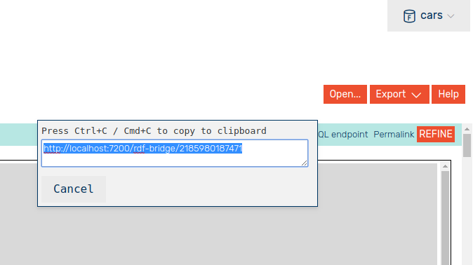
Click “SPARQL endpoint” and copy your endpoint (will be different) to be used later.
Reconciling the Data
If you have not done already, create a repository and head to the SPARQL tab.
You can see in the top right of this screenshot that I’m using a repository called “cars”.
In this query panel you want to copy the CONSTRUCT query we built and modify it a little. The full query is here:
PREFIX rdf: <http://www.w3.org/1999/02/22-rdf-syntax-ns#>
PREFIX rdfs: <http://www.w3.org/2000/01/rdf-schema#>
PREFIX dbo: <http://dbpedia.org/ontology/>
PREFIX dbp: <http://dbpedia.org/property/>
INSERT {
?car rdfs:label ?taggedname ;
rdf:type dbo:Company ;
dbo:location ?location .
?location rdf:type dbo:Country ;
rdfs:label ?lname ;
dbp:populationCensus ?pop .
} WHERE { SERVICE <http://localhost:7200/rdf-bridge/yourID> {
?c <urn:col:carNames> ?cname .
BIND(STRLANG(?cname, "en") AS ?taggedname)
SERVICE <https://dbpedia.org/sparql> {
?car rdfs:label ?taggedname ;
dbo:location | dbo:locationCountry ?location .
?location rdf:type dbo:Country ;
rdfs:label ?lname ;
dbp:populationCensus | dbo:populationTotal ?pop .
FILTER (LANG(?lname) = "en")
}}
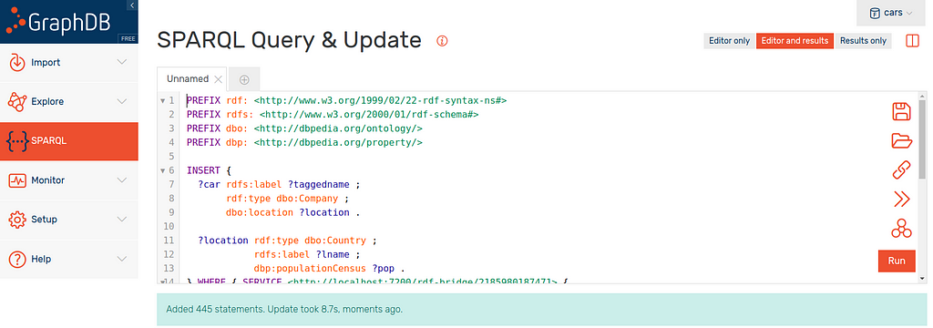
}The first thing we do is replace CONSTRUCT with INSERT as we now want to ingest the returned graph into our repository.
The next and final thing we must do is nest the entire WHERE clause into a second SERVICE tag. This time however, the service endpoint is the endpoint you copied at the end of the construction section.
This constructs the graph and inserts it into your repository!
It should be a much larger graph but the messiness of DBpedia strikes again! Many car manufacturers are connected to the string label of their location and not the entity. Therefore, the locations do not have a population and are consequently not returned.
We started with a small .csv of car manufacturer names so lets explore this graph we now have.
Exploring the New Graph
If we head to the “Explore” tab and view Japan for example, we can see our data.
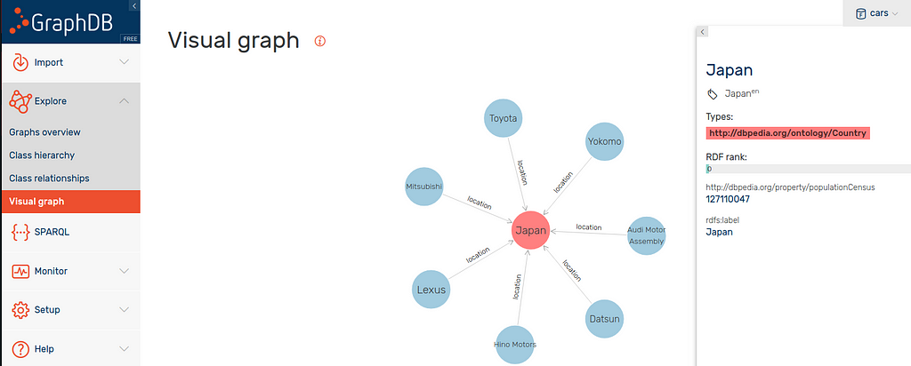
Japan has the attached type dbo:Country, label, population and has seven car manufacturers.
There is no point in linking data if we cannot gain further insight so lets head to the “SPARQL” tab of the workbench.
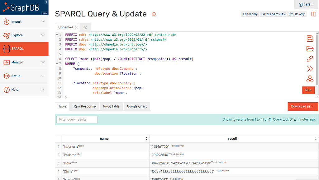
In this screenshot we can see the results of the below query. This query returns each country alongside the number of people per car manufacturer in that country.
There is nothing new in this query if you have read my SPARQL introduction. I have used the MAX population as some countries have two attached populations due to DBpedia.
PREFIX rdf: <http://www.w3.org/1999/02/22-rdf-syntax-ns#>
PREFIX rdfs: <http://www.w3.org/2000/01/rdf-schema#>
PREFIX dbo: <http://dbpedia.org/ontology/>
PREFIX dbp: <http://dbpedia.org/property/>
SELECT ?name ((MAX(?pop) / COUNT(DISTINCT ?companies)) AS ?result)
WHERE {
    ?companies rdf:type dbo:Company ;
               dbo:location ?location .

    ?location rdf:type dbo:Country ;
              dbp:populationCensus ?pop ;
              rdfs:label ?name .
}
GROUP BY ?name
ORDER BY DESC (?result)
In the screenshot above you can see that the results (ordered by result in descending order) are:
- Indonesia
- Pakistan
- India
- China
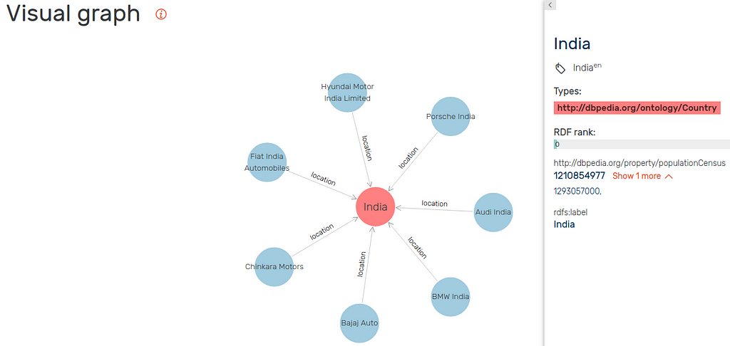
India of course has a much larger population than Indonesia but also has a lot more car manufacturers (as shown below).
If you were a car manufacturer in Asia, Indonesia might be a good market to target for export as it has a high population but very little local competition.
Conclusion
We started with a small list of car manufacturer names but, by using GraphDB and DBpedia, we managed to extend this into a small graph that we could gain actual insight from.
Of course, this example is not entirely useful but perhaps you have a list of local areas or housing statistics that you want to reconcile with mapping or government linked open data. This can be done using the above approach to help you or your business gain further insight that you could not have otherwise identified.
Linked Data Reconciliation in GraphDB was originally published in Wallscope on Medium, where people are continuing the conversation by highlighting and responding to this story.