
CONSTRUCT queries, VALUES and more property paths.
It was (quite rightly) pointed out that I strangely did not cover CONSTRUCT queries in my previous tutorial on Constructing SPARQL Queries. Additionally, I then went on to use CONSTRUCT queries in both my Transforming Tabular Data into Linked Data tutorial and the Linked Data Reconciliation article.
So, to finally correct this - I will cover them here!
Contents
SELECT vs CONSTRUCT
First Basic Example
- VALUES
- Alternative Property Paths
Second Basic Example
Example From the Reconciliation Article
Example From the Benchmark (Sneak Preview)
SELECT vs CONSTRUCT
In my last tutorial, I basically ran through SELECT queries from the most basic to some more complex. So what’s the difference?
With selects we are trying to match patterns in the knowledge graph to return results. With constructs we are specifying and building a new graph to return.
In the two tutorials linked (in the intro) I was constructing graphs from tabular data to then insert into a triplestore. I will discuss sections of these later but you should be able to follow the full queries after going through this tutorial.
We usually use CONSTRUCT queries at Wallscope to build a graph for the front-end team. Essentially, we create a portable sub-graph that contains all of the information needed to build a section of an application. Then instead of many select queries to the full database, these queries can be run over the much smaller sub-graph returned by the construct query.
First Basic Example
For this first example I will be querying my Superhero dataset that you can download here.
Each superhero entity in this dataset is connected to their height with the predicate dbo:height as shown here:
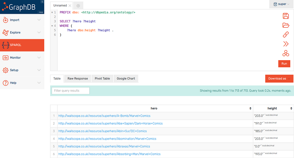
Using this basic SELECT query:
PREFIX dbo: <http://dbpedia.org/ontology/>
SELECT ?hero ?height
WHERE {
    ?hero dbo:height ?height .
}
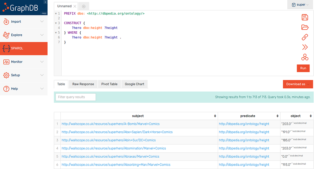
Now lets modify this query slightly into a CONSTRUCT that is almost the same:
PREFIX dbo: <http://dbpedia.org/ontology/>
CONSTRUCT {
    ?hero dbo:height ?height
} WHERE {
    ?hero dbo:height ?height .
}
As you can see, this returns the same information but in the form: subject, predicate, object.
This is obviously trivial and not entirely useful but we can play with this graph in the construct with only one condition:
All variables in the CONSTRUCT must be in the WHERE clause.
Basically, like in a SELECT query, the WHERE clause matches patterns in the knowledge graph and returns any variables. The difference with a CONSTRUCT is that these variables are then used to build the graph described in the CONSTRUCT clause.
Hopefully that is clear, but it makes more sense if we change the graph description.
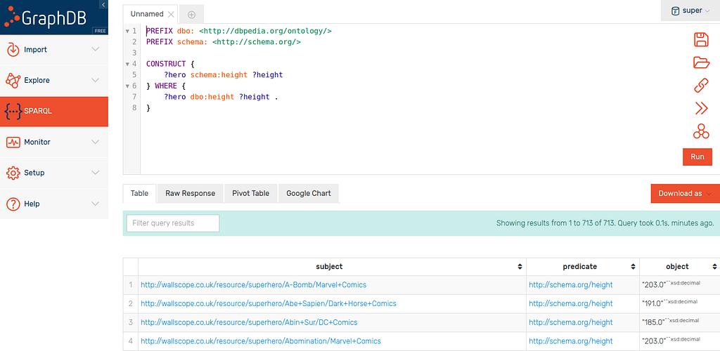
For example, if we decided that we wanted to use schema instead of DBpedia’s ontology, we could switch to it in the first clause:
PREFIX dbo: <http://dbpedia.org/ontology/>
PREFIX schema: <http://schema.org/>
CONSTRUCT {
    ?hero schema:height ?height
} WHERE {
    ?hero dbo:height ?height .
}
This then returns the superheroes attached to their heights with the schema:height predicate as the variables are matched in the WHERE clause and then recombined in the CONSTRUCT clause.
This simple predicate switching is not entirely useful on it’s own (unless you really need to switch ontology for some reason) but is a good first step to understand this type of query.
To create some more useful CONSTRUCT queries, I’ll first go through VALUES and another type of property path.
VALUES
I’m sure there are many use-cases in which the VALUES clause is incredibly useful but I can’t say that I use it often. Essentially, it allows data to be provided within the query.
If you are searching for a particular sport in a dataset for example, you could match all entities that are sports and then filter the results for it. This gets more complex however if you are looking for a few particular sports and you may want to provide the few sports within the query.
With VALUES you can constrain your query by creating a variable (can also create multiple variables) and assigning it some data.
I tend to use this with federated queries to grab data (usually for insertion into my database) about a few particular entities.
Let’s go through a practical example of this:
PREFIX dbr: <http://dbpedia.org/resource/>
SELECT ?country ?pop
WHERE {
    VALUES ?country {
        dbr:Scotland
        dbr:England
        dbr:Wales
        dbr:Northern_Ireland
        dbr:Ireland
    }
}
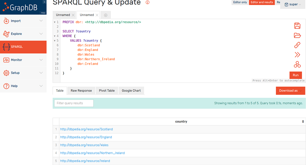
In this example I am interested in the five largest countries in the British Isles to compare populations. For reference (I’m from Scotland and had to check I was correct so imagine others may find this useful also):
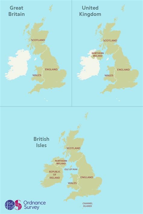
I am using DBpedia for this example so I have assigned the five country entities to the variable ?countries and selected them to be returned.
It should therefore be easy enough to grab the corresponding populations you’d think. I add the SERVICE clause to make this a federated query (covered previously). This just sends the countries defined within the query to DBpedia and returns their corresponding populations.
PREFIX dbr: <http://dbpedia.org/resource/>
PREFIX dbp: <http://dbpedia.org/property/>
SELECT ?country ?pop
WHERE {
    VALUES ?country {
        dbr:Scotland
        dbr:England
        dbr:Wales
        dbr:Northern_Ireland
        dbr:Ireland
    }

    SERVICE <http://dbpedia.org/sparql> {
        ?country dbp:populationCensus ?pop .
    }
}
Here are the results:
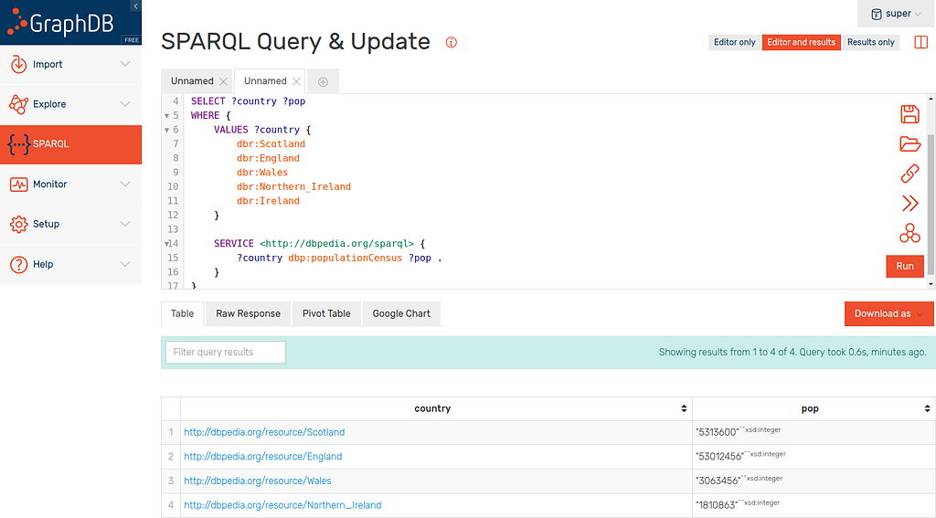
You will notice however that Ireland is missing from the results! You will often find this kind of problem with linked open data, the structure is not always consistent throughout.
To find Ireland’s population we need to switch the predicate from dbp:populationCensus to dbo:populationTotal like so:
PREFIX dbr: <http://dbpedia.org/resource/>
PREFIX dbo: <http://dbpedia.org/ontology/>
SELECT ?country ?pop
WHERE {
    VALUES ?country {
        dbr:Scotland
        dbr:England
        dbr:Wales
        dbr:Northern_Ireland
        dbr:Ireland
    }

    SERVICE <http://dbpedia.org/sparql> {
        ?country dbo:populationTotal ?pop .
    }
}
which returns Ireland alongside its population… but none of the others:
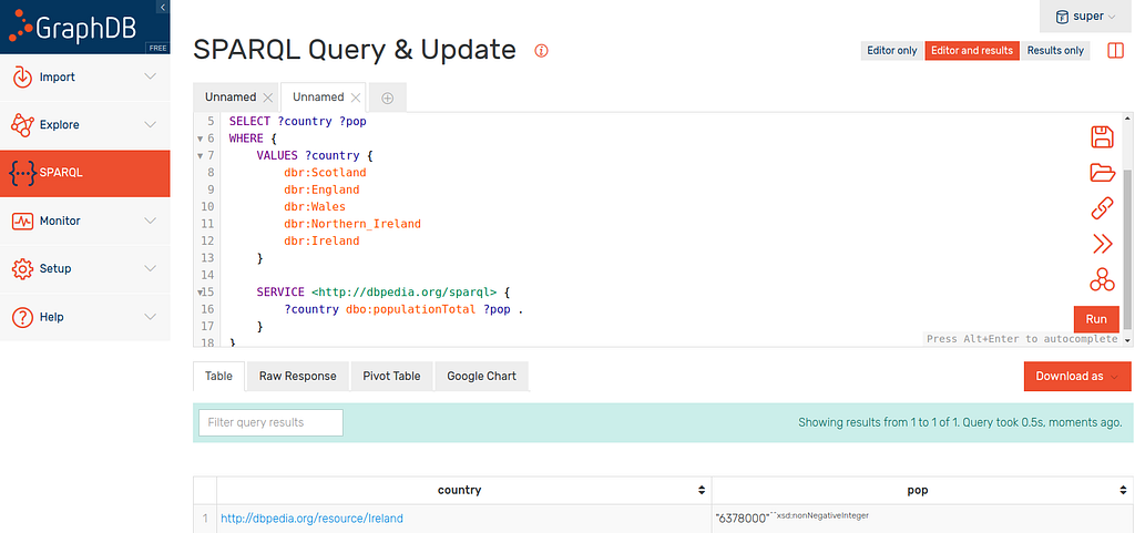
This is of course a problem but before we can construct a solution, let’s run through alternate property paths.
Alternative Property Paths
In my last SPARQL tutorial we covered sequential property paths which (once the benchmark query templates come out) you may notice I am a big fan of.
Another type of property path that I use fairly often is called the Alternative Property Path and is made use of with the pipe (|) character.
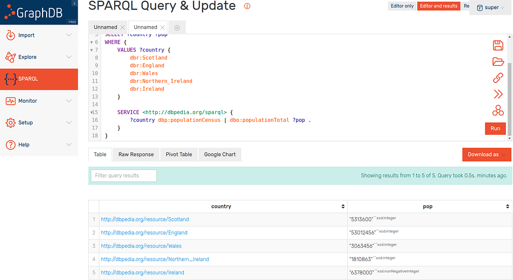
If we look back at the problem above in the VALUES section, we can get some populations with one predicate and the rest with another. The alternate property path allows us to match patterns with either! For example, if we modify the population query above we get:
PREFIX dbr: <http://dbpedia.org/resource/>
PREFIX dbp: <http://dbpedia.org/property/>
PREFIX dbo: <http://dbpedia.org/ontology/>
SELECT ?country ?pop
WHERE {
    VALUES ?country {
        dbr:Scotland
        dbr:England
        dbr:Wales
        dbr:Northern_Ireland
        dbr:Ireland
    }

    SERVICE <http://dbpedia.org/sparql> {
        ?country dbp:populationCensus | dbo:populationTotal ?pop .
    }
}
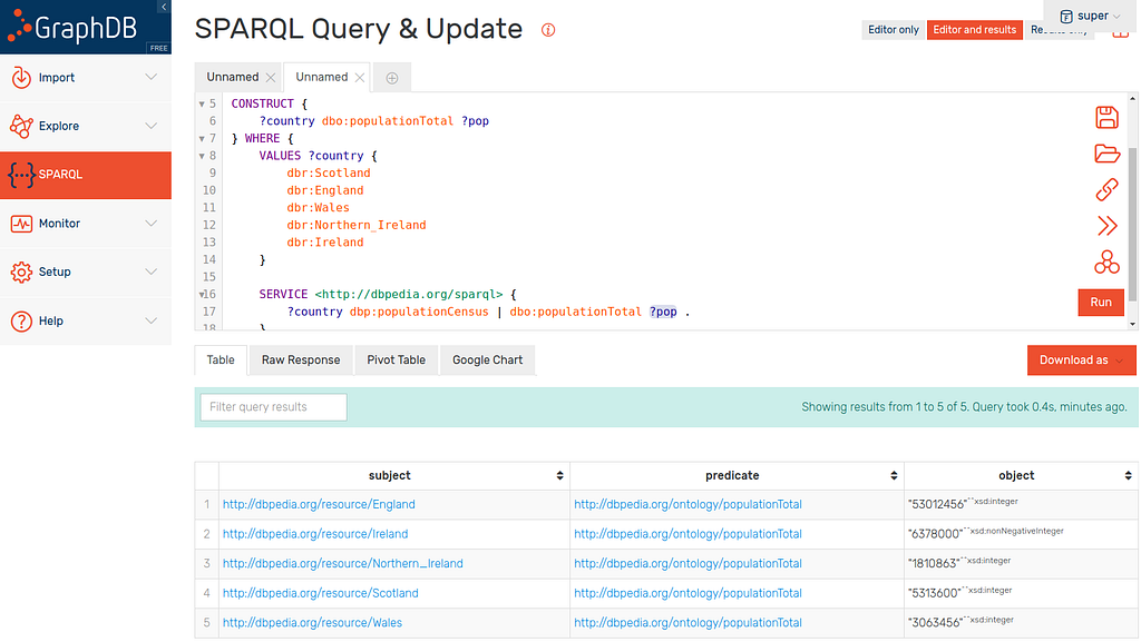
This is such a simple change but so powerful as we now return every country alongside their population with one relatively basic query:
This SELECT is great if we are just looking to find some results but what if we want to store this data in our knowledge graph?
Second Example
It would be a hassle to have to use this alternative property path every time we want to work with country populations. In addition, if users were not aware of this inconsistency, they could find and report incorrect results.
This is why we CONSTRUCT the result graph we want without the inconsistencies. In this case I have chosen dbo:populationTotal as I simply prefer it and use that to connect countries and their populations:
PREFIX dbr: <http://dbpedia.org/resource/>
PREFIX dbp: <http://dbpedia.org/property/>
PREFIX dbo: <http://dbpedia.org/ontology/>
CONSTRUCT {
    ?country dbo:populationTotal ?pop
} WHERE {
    VALUES ?country {
        dbr:Scotland
        dbr:England
        dbr:Wales
        dbr:Northern_Ireland
        dbr:Ireland
    }

    SERVICE <http://dbpedia.org/sparql> {
        ?country dbp:populationCensus | dbo:populationTotal ?pop .
    }
}
This query returns the countries and their populations like we saw in the previous section but then connects each country to their population with dbo:populationTotal as described in the CONSTRUCT clause. This returns consistent triples:
This is useful if we wish to store this data as the fact it’s consistent will help avoid the problems mentioned above. I used this technique in one of my previous articles so lets take a look.
Example From Reconciliation Tutorial
This example is copied directly from my data reconciliation tutorial here. In that article I discuss this query in a lot more detail.
In brief, what I was doing here was grabbing car manufacturer names from tabular data and enhancing that information to store and analyse.
PREFIX rdf: <http://www.w3.org/1999/02/22-rdf-syntax-ns#>
PREFIX rdfs: <http://www.w3.org/2000/01/rdf-schema#>
PREFIX dbo: <http://dbpedia.org/ontology/>
PREFIX dbp: <http://dbpedia.org/property/>
CONSTRUCT {
  ?car rdfs:label ?taggedname ;
       rdf:type dbo:Company ;
       dbo:location ?location .

  ?location rdf:type dbo:Country ;
            rdfs:label ?lname ;
            dbp:populationCensus ?pop .
} WHERE {
  ?c <urn:col:carNames> ?cname .

  BIND(STRLANG(?cname, "en") AS ?taggedname)

  SERVICE <https://dbpedia.org/sparql> {

    ?car rdfs:label ?taggedname ;
         dbo:location | dbo:locationCountry ?location .

    ?location rdf:type dbo:Country ;
              rdfs:label ?lname ;
              dbp:populationCensus | dbo:populationTotal ?pop .

    FILTER (LANG(?lname) = "en")
  }
}
There is little point repeating myself here so if interested, please take a look. What I am trying to display here is that I have used both the alternative property path (twice!) and the CONSTRUCT clause previously in an example use-case.
Construct queries are perfectly suited to ensuring any data you store is well typed, structured and importantly consistent.
I have been short on time since starting my new project but I am still working on the benchmark in development.
Example From The Benchmark (Sneak Preview)
The benchmark repository is not yet public as I don’t want opinions to be formed before it is fleshed out a little more.
I thought it would be good however to give a real (not made for a tutorial) example query that uses what this article teaches:
PREFIX dbo: <http://dbpedia.org/ontology/>
PREFIX schema: <http://schema.org/>
PREFIX dbp: <http://dbpedia.org/property/>
INSERT {
    ?city dbo:populationTotal ?pop
} WHERE {
    {
      SELECT ?city (MAX(?apop) AS ?pop) {
          ?user schema:location ?city .

          SERVICE <https://dbpedia.org/sparql> {
            ?city dbo:populationTotal | dbp:populationCensus ?apop .
          }
      }
      GROUP BY ?city
    }
}
You will notice that this does not contain the CONSTRUCT clause but INSERT instead. You will see me do this switch in both the articles I linked in the introduction. Basically this does nothing too different, the graph that is constructed is inserted into your knowledge graph instead of just returned. The same can be done with the DELETE clause to remove patterns from your knowledge graph.
This query is very similar to the examples throughout this article (by design of course) but grabs countries populations from DBpedia and inserts them into the graph. This is just one point within the query cycle at which the graph changes structure in the benchmark.
Finally, the MAX population is grabbed because some countries in DBpedia have two different populations attached to them…
Conclusion
Hopefully this is useful for some of you! We have covered why and how to use construct queries along with values and alternative property paths.
At the end of May I am going to the DBpedia community meeting in Leipzig so my next linked data article will likely cover things I learned at that event or progress on the benchmark development.
In the meantime I will be releasing my next Computer Vision article and another dive into natural conversation.
Constructing More Advanced SPARQL Queries was originally published in Wallscope on Medium, where people are continuing the conversation by highlighting and responding to this story.