Second Example

In Section 4.3 we showed a very simple AUTO CLUI script, in this Section we will describe a more complex example, which introduces several new AUTO CLUI commands as well as some basic Python  constructs for conditionals and looping. We will not provide an exhaustive reference for the Python  language, but only the very basics. For more extensive documentation we refer the reader to Lut:96 Lut:96 or the web page http://www.python.org. In this section we will describe each line of the script in detail, and the full text of the script is in Figure 4.7.

The script begins with a section, extracted into Figure 4.8, which performs a task identical to that shown in Figure 4.2 except that the shorthand discussed in Section 4.3 is used for the ld command.

The next section of the script, extracted into Figure 4.9, introduces three new AUTO CLUI commands. First, sv('bvp') (Section 4.14.6 in the reference) saves the results of the AUTO run into files using the base name bvp and the filename extensions in Table 4.3. For example, in this case the bifurcation diagram file fort.7 will be saved as b.bvp, the solution file fort.8 will be saved as s.bvp, and the diagnostics file fort.9 will be saved as d.bvp. Next, ld(s='bvp') loads the solution file s.bvp into memory so that it can be used by AUTO for further calculations.

Up to this point all of the commands presented have had analogs in the command language discussed in Section 5, and the AUTO CLUI has been designed in this way to make it easy for users to migrate from the old command language to the AUTO CLUI. The next command, namely data = sl('bvp') (Section 4.14.19 in the reference) is the first command which has no analog in the old command language. The command sl('bvp') parses the file s.bvp and returns a python object which encapsulates the information contained in the file and presents it to the user in an easy to use format. Accordingly, the command data = sl('bvp') stores this easy to use representation of the object in the Python  variable data. Note, variables in Python  are different from those in languages such as C in that their type does not have to be declared before they are created. Finally, ch("NTST",50) (Section 4.14.32 in the reference) changes the NTST value to 50 (see Section 10.2.1). To be precise, the command ch("NTST",50) only modifies the ``in memory'' version of the AUTO constants created by the ld('bvp') command. The original file c.bvp is not modified.

The next section of the script, extracted into Figure 4.10, shows as example of looping and conditionals in an AUTO CLUI script. The first line for solution in data: is the Python  syntax for loops. The data variable was defined in Figure 4.9 to be the parsed version of an AUTO fort.8 file, and accordingly contains a list of the solutions from the fort.8 file. The command for solution in data: is used to loop over all solutions in the data variable by setting the variable solution to be one of the solutions in data and then calling the rest of the code in the block.

Python  differs from most other computer languages in that blocks of code are not defined by some delimiter, such as {} in C, but by indentation. In Figure 4.7 the commands plot('bvp') and wait() are not part of the loop, because they are indented differently. This can be confusing first time users of Python , but it has the advantage that the code is forced to have a consistent indentation style.

The next command in the script, if solution["Type name"] == "BP": is a Python  conditional. It examines the contents of the variable solution (which is one of the entries in the array of solutions data) and checks to see if the condition solution["Type name"] == "BP" holds. For parsed fort.8 files Type name BP corresponds to a bifurcation point. Accordingly, the function of this loop and conditional is to examine every solution in the fort.8 file and run the following commands if the solution is a bifurcation point.

The next line is ch("IRS", solution["Label"]) which changes the ``in memory'' version of the AUTO constants file to set IRS (see Section 10.8.5) equal to the label of the bifurcation point. We then use ch("ISW", -1) to change the AUTO constant ISW to -1, which indicates a branch switch (see Section 10.8.3).

We then use a run() command to perform the calculation of the bifurcating branch and then append the data to the s.bvp, b.bvp, and d.bvp files with the ap('bvp') command (Section 4.14.1 in the reference). In addition, as can be seen in Figure 4.10, the # character is the Python  comment character. When the Python  interpretor encounters a # character it ignores everything from that character to the end of the line.

Finally, we us ch("DS",-pr("DS")) to change the AUTO initial step size from positive to negative, which allows us to compute the bifurcating branch in the other direction (see Section 10.5.1). Running the AUTO calculation with the run() command and appending the data the appropriate files with the ap('bvp') command completes the body of the loop.

Now that the section of script shown in Figure 4.10 has finished computing the bifurcation diagram, the command plot('bvp') brings up a plotting window (Section 4.14.20 in the reference), and the command wait() causes the AUTO CLUI to wait for input. You may now exit the AUTO CLUI by pressing any key in the window in which you started the AUTO CLUI.

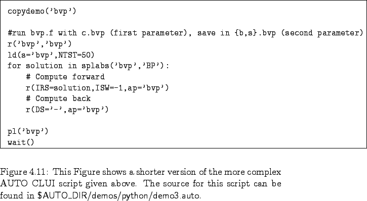
For convenience, some of these commands have shorter forms. For instance, you can directly specify a change of NTST in the ld and run commands, by giving NTST=xxx as an extra parameter, as well as the special DS='-' notation to quickly revert the direction (the sign of DS). The command run also accepts the files to save or append to using sv= and ap=, respectively. Another helpful function is splabs, that return a list of labels for a given solution file. A shorter version of the complex AUTO  CLUI script is given in Figure 4.11.