brc : Chebyshev Collocation in Space.

This demo illustrates the computation of stationary solutions and periodic solutions to systems of parabolic PDEs in one space variable, using Chebyshev collocation in space. More precisely, the approximate solution is assumed of the form $u(x,t) = \sum_{k=0}^{n+1} u_k(t) \ell_k(x)$. Here $u_k(t)$ corresponds to $u(x_k,t)$ at the Chebyshev points $\bigl\{ x_k \bigr\}_{k=1}^{n}$ with respect to the interval $[0,1]$. The polynomials $\bigl\{ \ell_k(x) \bigr\}_{k=0}^{n+1}$ are the Lagrange interpolating coefficients with respect to points $\bigl\{ x_k \bigr\}_{k=0}^{n+1}$, where $x_0=0$ and $x_{n+1}=1$. The number of Chebyshev points in $[0,1]$, as well as the number of equations in the PDE system, can be set by the user in the file brc.inc.

As an illustrative application we consider the Brusselator (HoKnKu:87 HoKnKu:87)

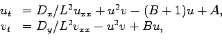
$$\begin{array}{cl} u_t &= {D_x / L^2} u_{xx} + u^2v - (B+1)u + A, \\ v_t &= {D_y / L^2} v_{xx} - u^2v + Bu, \\ \end{array}$$ (16.3)

with boundary conditions $u(0,t)=u(1,t)=A$ and $v(0,t)=v(1,t)=B/A$.

Note that, given the non-adaptive spatial discretization, the computational procedure here is not appropriate for PDEs with solutions that rapidly vary in space, and care must be taken to recognize spurious solutions and bifurcations.

Table 16.4: Commands for running demo brc.

AUTO -COMMAND	ACTION
! mkdir brc	create an empty work directory
cd brc	change directory
demo('brc')	copy the demo files to the work directory
run(c='brc.1')	compute the stationary solution family with Hopf bifurcations
sv('brc')	save output-files as b.brc, s.brc, d.brc
run(c='brc.2',s='brc')	compute a family of periodic solutions from the first Hopf point. Constants changed : IRS, IPS
ap('brc')	append the output-files to b.brc, s.brc, d.brc
run(c='brc.3',s='brc')	compute a solution family from a secondary periodic bifurcation. Constants changed : IRS, ISW
ap('brc')	append the output-files to b.brc, s.brc, d.brc