bru : Euler Time Integration (the Brusselator).

This demo illustrates the use of Euler's method for time integration of a nonlinear parabolic PDE. The example is the Brusselator (HoKnKu:87 HoKnKu:87), given by

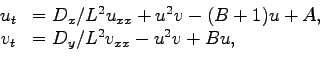$$\begin{array}{cl} u_t &= {D_x / L^2} u_{xx} + u^2v - (B+1)u + A, \\ v_t &= {D_y / L^2} v_{xx} - u^2v + Bu, \\ \end{array}$$ (16.5)

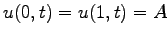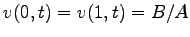with boundary conditions $u(0,t)=u(1,t)=A$ and $v(0,t)=v(1,t)=B/A$. All parameters are given fixed values for which a stable periodic solution is known to exist.

The continuation parameter is the independent time variable, namely PAR(14). The AUTO -constants DS, DSMIN, and DSMAX then control the step size in space-time, here consisting of PAR(14) and $(u(x),v(x))$. Initial data at time zero are $u(x)=A - 0.5 \sin(\pi x)$ and $v(x)=B/A + 0.7 \sin(\pi x)$. Note that in the subroutine STPNT the space derivatives of $u$ and $v$ must also be provided; see the equations-file bru.f.

Euler time integration is only first order accurate, so that the time step must be sufficiently small to ensure correct results. This option has been added only as a convenience, and should generally be used only to locate stationary states. Indeed, in the case of the asymptotic periodic state of this demo, the number of required steps is very large and use of a better time integrator is advisable.

Table 16.6: Commands for running demo bru.

AUTO -COMMAND	ACTION
! mkdir bru	create an empty work directory
cd bru	change directory
demo('bru')	copy the demo files to the work directory
run(c='bru.1')	time integration
sv('bru')	save output-files as b.bru, s.bru, d.bru