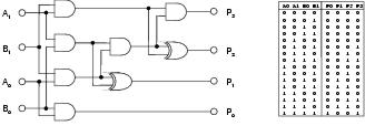
Figure 9.1: Two-bit multiplier problem. Truth table and standard solution.
This chapter presents the results of a series of experiments designed to give insight into the performance, behaviour, and scope of enzyme genetic programming. In particular, this chapter aims to document:
The implementation of enzyme GP used for this study uses a number of metrics to measure performance and behaviour. Table 9.1 lists those which are referred to in this chapter. Table 9.2 lists the parameters of the system, along with their default values. Where no parameter value is given for a particular experiment, the default value is assumed. Fitness values and run lengths are typically not normally distributed and where statistical significance is given, these are the results of non-parametric Mann-Whitney or Kruskal-Wallis tests. Variances and actual values reported by statistical tests are generally not given to avoid clutter. A confidence level of 95% is used to determine statistical significance.
| Metric | Range | Description |
| Computational effort | 0+ | Number of evaluations required to produce a 99% probability of finding an optimal solution |
| Distance | 0%-100% | Average distance, as a proportion of a dimension, between the functionality of a binding site and its substrate |
| Expression | 0%-100% | Proportion of functional components which are currently expressed |
| Fitness | -0 | Highest fitness found within a population, measured by number of incorrect output bits during simulation |
| Genetic linkage | 0%-100% | Genetic distance between interacting components as a proportion of genome length |
| Output distance | 0%-100% | Distance between an output terminal's binding site and its substrate |
| Program size | 0+ | Number of functional components expressed within a program |
| Representation length | 0+ | Number of functional components within a representation |
| Reuse | 0+ | Number of times a single component is bound during program development |
| Solution time | 0+ | Number of generations required to find an optimal solution |
| Success rate | 0%-100% | Proportion of runs which found an optimal solution |
Table 9.1: Metrics used to measure performance and behaviour of program evolution.
| Parameter Name | Label | Default value |
| Crossover type | transfer and remove | |
| Development strategy | top-down | |
| Distance limit for gene alignment in uniform crossover | 1 | |
| Functionality dimension initialisation power | i | 3 |
| Generation limit | l | 200 |
| Number of binding sites per input component | bs | 3 |
| Number of runs per data point | r | 50 |
| Phenotypic linkage learning rate | llr | 0% |
| Population dimensions | pd | 18 x 18 |
| Problem | 2-bit multiplier | |
| Proportion of gene pairs recombined in uniform crossover | 15% | |
| Rate of activity mutation | ma | 1.5% |
| Rate of binding site strength mutation | ms | 2% |
| Rate of functionality dimension mutation | mf | 2% |
| Shape input bias (from equation 8.1) | k | 0.3 |
| Transfer size upper limit for TR crossover | tu | 5 |
Table 9.2: Behavioural parameters and their default settings.
All the experiments reported in this chapter use symbolic regression as a problem domain. Application is limited to discrete regression problems involving Boolean logic. Whilst this might limit the generality of the results, these problems were chosen for their relative difficulty with regard to recombinative search.
Symbolic regression involves the inference of a symbolic expression from a representative set of < input,output > data points. For Boolean regression problems, these data points can be interpreted as a conventional truth table of the kind used in combinational logic design. All the problems used in this study are specified by complete truth tables: providing output test cases for every possible combination of inputs. For a particular problem, expressions can be built from members of a pre-defined non-terminal set, which specifies the available Boolean logic functions; and a terminal set, which specifies the available inputs. Test problems are listed in Table 9.3. A standard solution for the two-bit multiplier problem is shown in figure 9.1.
Figure 9.1: Two-bit multiplier problem. Truth table and standard solution.
| Name | Inputs | Outputs | Function set |
| 1-bit full adder | 3 | 2 | AND,OR,XOR |
| 2-bit full adder | 5 | 3 | XOR,MUX |
| 2-bit multiplier | 4 | 4 | AND,XOR |
| 3-bit multiplier | 6 | 6 | AND,XOR |
| even-3-parity | 3 | 1 | AND,OR,NAND,NOR |
| even-4-parity | 4 | 1 | AND,OR,NAND,NOR |
Table 9.3: Boolean regression test problems.
Similar Boolean regression problems have also been addressed by Miller et al. [2000], Coello et al. [2002], and Koza [1992] using various forms of GP. Vassilev et al. [1999] have carried out an analysis of various multiplier landscapes and have found them to be typified by large planes of equal-valued solutions and little fitness gradient information. This would appear to be typical of Boolean regression landscapes and implies that such problems are difficult to solve using recombination; a view which is also expressed in [Miller et al., 2000].
| ||||||||||||||||||||||||
| ||||||||||||||||||||||||
| ||||||||||||||||||||||||
| ||||||||||||||||||||||||
Table 9.4: Performance of enzyme GP with different operators, recording average solution time, success rate, and computational effort (CE).
Table 9.4 shows the performance of enzyme GP upon a selection of problems. The adder, multiplier and even-4-parity problems have been solved by Miller et al. [2000] using Cartesian GP. Results from Koza [Koza, 1992,Koza, 1994], using tree-based GP, are available for both parity problems. Koza [1992] has also attempted the 2-bit adder problem, but quantitative results are not available. Miller records minimum computational effort21 of between 210,015 and 585,045 for the 2-bit multiplier problem. Enzyme GP, requiring a minimum computational effort of 136,080 for a population of 324, compares favourably with these results. For the 2-bit adder problem, Miller cites a minimum computational effort of 385,110. For enzyme GP, using the same functions as Miller, mimimum effort is 244,620: also a favourable comparison.
Koza has evolved even-n-parity circuits using populations of size 4,000 [Koza, 1992] and 16,000 [Koza, 1994]. For the even-3-parity problem (and without using ADFs), this gives minimum computational efforts of 80,000 and 96,000 respectively. For the even-4-parity problem, minimum computational efforts are 1,276,000 and 384,000 respectively. For enzyme GP, minimum computational effort has been calculated at 79,000 for the even-3-parity problem with a population of 100. For the even-4-parity problem with a population of 625, minimum computational effort is 2,703,000 with crossover and 1,830,000 without. This suggests that enzyme GP cannot easily evolve even-n-parity circuits where n > 3, at least for these (relatively small) population sizes and especially when crossover is used. This agrees with Miller's findings, where only 15 correct even-4-parity circuits were found in the course of 400 million evaluations. Langdon and Poli [1998] have suggested that parity circuits are unsuitable benchmarks for GP. Furthermore, parity circuits involve a high-degree of structure re-use and it seems plausible that sub-tree crossover, which is able to transfer sub-structures independently of their original context, may be more able to develop this sort of pattern than enzyme GP.
 |
|
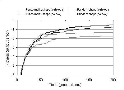
Figure 9.2: Comparing mean number of output bit errors when evolving two-bit multipliers for functionality shapes and random shapes with and without TR recombination (c/o).
The results outlined above suggest that enzyme GP is able to compete favourably against GPs which use indirect context representations. However, given the differences in evolutionary frameworks and other implementation details, it is difficult to compare indirect and implicit context by comparing the performance of different GP systems. A more direct comparison between indirect and implicit context representations can be made by comparing the performance of enzyme GP with functionality shapes against enzyme GP with randomly generated shapes. These random shapes effectively specify an indirect context, where there is no relationship between pattern and behaviour. Figure 9.2 shows that fitness for enzyme GP with random shapes initially grows at a high rate, but falls to a relatively low rate once a certain fitness level is reached. This suggests a high level of disruptive variation, which initially benefits search but later becomes a hindrance to effective exploitation. Enzyme GP with functionality shapes, by comparison, demonstrates a steady rate of decay in fitness growth, indicating a more structured search which continues until the optimum is found. The performance statistics listed in figure 9.2 indicate that performance is considerably better with functionality shape than with random shape22. This supports the notion that implicit context captures more meaningful context than indirect context.
 |
|
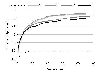
Figure 9.3: Comparing fitness evolution and performance for different ratios of activity to binding sites during shape calculation.
According to equation 8.1, a component's shape is a weighted sum of the functionality of its activity and the functionalities declared by its binding sites. Figure 9.3 shows the effect of this ratio upon fitness and performance: indicating that the best performance is attained when shape is calculated in an equal ratio from activity and binding sites. If shape calculation is weighted too far towards either activity or binding sites, then search becomes impaired. If the binding sites contribution is removed from shape calculation, then search becomes ineffective. If the activity contribution is removed, then performance becomes substantially degraded. These observations are not surprising. Weighting shape calculation too far towards the binding sites causes activity information, and therefore context information, to be lost. Weighting shape calculation too far towards activity causes the component's behavioural information to be lost; making it difficult to distinguish between the roles of components which have the same activity.
|
|
|
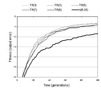
Figure 9.4: Comparing uniform and TR recombination. [Left] Fitness evolution for different transfer limits (TR) and size bounds (uniform). [Right] Ability to generate fitter programs and explore novel programs.
Section 8.6.1 described two types of recombination: uniform crossover and transfer and remove (TR). Table 9.4 shows that with the exception of the even-4-parity problem, the computational effort using uniform crossover is less than using TR crossover. However, this comparison is misleading since uniform crossover is constrained by size bounds whereas TR recombination is not. Uniform crossover, therefore, explores a smaller area of the search space; an area which, in these cases, is known to contain an optimal solution. Figure 9.4 shows more meaningful comparisons between these two kinds of recombination. The graph on the left of the figure plots fitness evolution for different operator parameter settings. It can be seen that whilst uniform crossover appears to compete favourably for the size bounds used in table 9.4, its performance becomes considerably impaired when size bounds are used which more accurately reflect the region explored by TR recombination. The graph on the right of figure 9.4 plots the evolution of recombination's ability to generate neutral and fitter solution variants. For both measures, the performance of TR recombination is significantly higher than uniform crossover. Notably, uniform crossover is far less able to explore neutral variants than TR crossover - suggesting that uniform crossover is too disruptive to search in the neighbourhood of existing solutions. This is unsurprising given that uniform crossover targets multiple sections of the representation and always causes components to be replaced rather than appended. TR recombination is used for most of the remaining experiments documented in this chapter: both for the above reasons and because it is computationally less expensive, behaviourally more interesting, and fairly insensitive to initial representation size and transfer size (as indicated by figure 9.4).
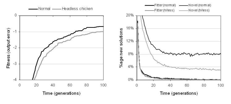
Figure 9.5: Comparing TR recombination against headless chicken TR recombination.
According to the arguments described in [Vassilev et al., 1999], recombination would be expected to offer relatively poor performance upon Boolean symbolic regression problems. For this reason, recombination was not used in Miller's experiments on digital circuit evolution [Miller et al., 2000]. However, results from experiments using enzyme GP indicate that recombination can play an important role in digital circuit evolution and, significantly, offers better search performance than mutation operators. Table 9.4 shows that, in all but the even-4-parity problem, enzyme GP with recombination performs considerably better than enzyme GP with mutation alone. In previous GP studies, headless chicken crossover operators, which recombine existing solutions with randomly generated solutions, have been used to show that crossover performs no better than macro-mutation. Results depicted in figure 9.5 show that for enzyme GP, TR recombination offers better performance than a headless chicken operator based upon TR recombination. This suggests that recombination is transferring useful information between programs. However, even the headless variant offers reasonable performance.
A more direct comparison between the search performance of recombination and mutation has been carried out by configuring enzyme GP's evolutionary framework to generate one child via recombination and another via mutation for every reproduction event and by measuring the relative fitness of the children produced by each operator. This was done for both functionality and random shapes.
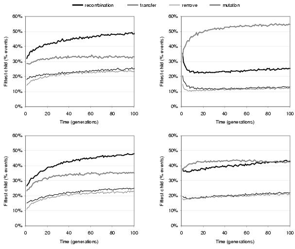
Figure 9.6: Comparing relative ability of recombination and mutation operators to generate fitter children during the evolution of [top] two-bit multipliers and [bottom] two-bit adders using [left] functionality shapes and [right] random shapes.
Figure 9.6 shows that when functionality shapes are used, recombination is responsible for generating the fittest child during a substantially greater proportion of reproduction events than mutation. This suggests that recombination has considerably more influence upon search than mutation. However, when random shapes are used, recombination is no longer the dominant operator with (especially for the multiplier problem) mutation generating the greater proportion of fitter children during reproduction events. This lends weight to the argument that implicit context improves the behaviour of recombination with respect to indirect context. Figure 9.6 also shows that transfer operations have a slightly higher success rate than remove operations during TR recombination. This reflects the fact that solutions are more likely to be disrupted by removing components than they are by gaining components.
The implementation of enzyme GP used for this study allows evolutionary behaviours to be observed at the level of individual solutions and individual variation events. Whilst these observations do not have the statistical significance of the macroscopic measures used elsewhere in this chapter, they provide an interesting insight into how evolution occurs at a microscopic level.
There are many kinds of behaviours which can occur as a consequence of applying variation operators. Nevertheless, many of these are built upon a selection of fairly simple behaviours which are seen to occur frequently within evolving populations. Figures 9.7 and 9.8 show examples of such behaviours that occur when transfer and remove operations are applied during recombination. The transfer operation cannot directly replace any components within a program representation (other than outputs). However, as figure 9.7 illustrates, it can still lead to behaviours at the program level that look like replacement. This happens because the new component has subsumed the role of the former component, offering a closer match to the input context declared by the parent node. Nevertheless, the former component is still present within the program representation and, if the new component were to be removed, could resume its former role in the program. Figure 9.7 also shows how subsumption is able to preserve the behaviour of the program below the component that has been replaced, indicating that the new component has a functionality similar to that of the former component, and illustrating the context preserving nature of recombination in enzyme GP.
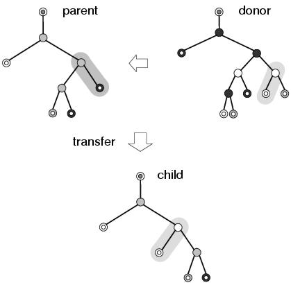
Figure 9.7: A simple example of subsumption resulting from a transfer operation. Different node and terminal shades represent different members of the function and terminal sets.
Figure 9.8 shows two other behaviours which often occur during recombination: insertion and deletion. In the example on the left of the figure, a transfer operation leads to a new sub-tree being inserted between two existing components, something which is not possible using sub-tree swapping recombination in standard GP. Again, the existing sub-tree below the root of the inserted sub-tree is preserved, and from the perspective of the component (the output terminal) above the inserted sub-tree, the new context is related to the former context: and presumably a closer fit to the implicit context declared by its binding site. In fact, insertion is a special case of subsumption where the subsuming component happens to declare an input context which matches the role of the component that it subsumed. In the other two example in figure 9.8, removal operations lead to parts of programs being deleted. In the example in the centre, two sub-trees are affected by a single removal operation. This shows how recombination operators in enzyme GP operate upon groups of components at the representation level rather than structures (in this case sub-trees) at the program level: a behaviour which is presumably more disruptive, but also more expressive, than conventional sub-tree crossover. In the example on the right of the figure, an entire sub-tree is removed from between two nodes. This is the complement of the behaviour which occurs in the transfer example on the left of the figure, and shows how a subsumption operation might be reversed. In both of these removal examples, the program below the deletion remains unaffected, showing how the remove operation also encourages context preservation.
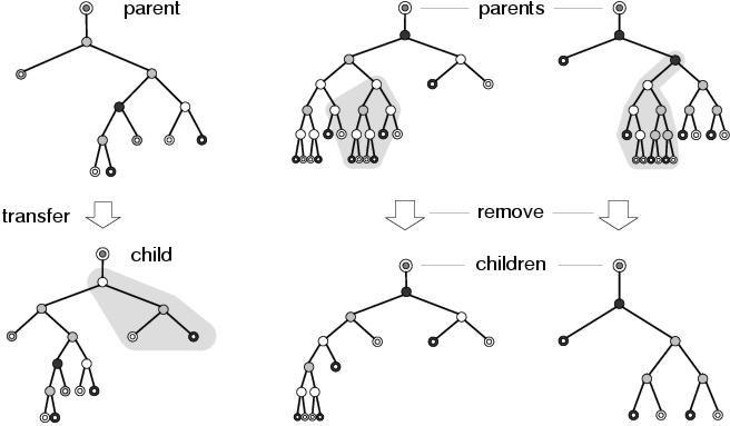
Figure 9.8: Behaviours resulting from transfer and remove operations.
Conceptually, all the components defined in a representation occupy some position in a subsumption hierarchy. At the top are the expressed components: those which appear in the program. Below these are any redundant copies of the expressed components. Below these are components that have been subsumed by the expressed components; and further down, components that were subsumed by components further up the hierarchy which have since themselves also been subsumed. At the bottom are components which have never been expressed but which could in principle be expressed if all the components above them in the subsumption hierarchy were removed. All the behaviours that occur in enzyme GP are a result of variation operators modifying this subsumption hierarchy: either by adding new entries, by removing entries or by re-ordering existing entries (which is what mutation operators are essentially doing). Nevertheless, the operators are not aware of this subsumption hierarchy. They blindly add, remove and re-order entries - only causing change in the program when they happen to add, remove or re-order entries at the top of the hierarchy. All other changes are absorbed into the lower echelons of the hierarchy. Subsumption supports the idea that the program representation used by enzyme GP promotes meaningful variation filtering: since it is clearly the way in which the representation describes the program, rather than the action of the variation operators, that allows subsumptive behaviours to occur.
 |
 |
 |
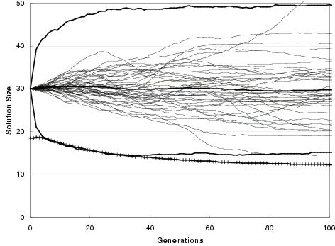 |
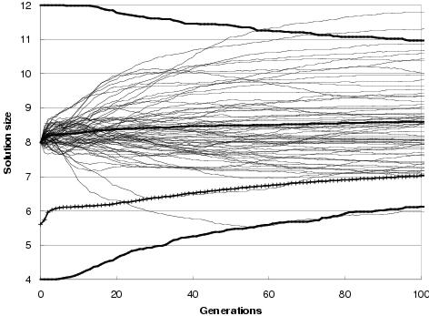
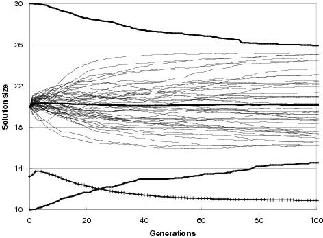
Figure 9.9: Two-bit multiplier size evolution using [top] uniform crossover and [bottom] TR recombination. Faint lines show average representation sizes for each run. Heavy un-crossed lines show average minimum, average and maximum representation sizes across all runs. Heavy crossed line shows average program size across all runs. Minimum optimal program size for this problem is 7 gates.
In general, enzyme GP produces little or no bloat in both representation and program size. Figure 9.9 shows the size evolution of two-bit multipliers for both recombination operators and for different initial representation sizes. Size evolution under TR recombination is of particular interest, since in principal there is no upper bound to solution length. Nevertheless, there appears to be little pressure for the recombination operators to explore representation lengths much larger than the initial representation length. What little amount of growth there is for an initial representation length of 15 components can readily be accounted for either by the differential performance of the transfer and remove operators23, by an initial representation length insufficient to easily express optimal solutions, or by there being many more solution representations of greater length than the initial representation length (or shorter). However, for an initial representation length of 30 components, even these factors appear to have no effect upon representation length.
Figure 9.9 also shows that program size evolution is not proportional to representation length evolution. For both forms of recombination, change in average program size does not reflect change in average representation length. For TR recombination: with an initial representation length of 15 components, whilst representation length grows on average over the course of a run, program size remains fairly stable. For an initial representation length of 30, average program size falls whereas representation length remains stable. This behaviour reflects a decoupling between program and representation; and is an expected consequence of using an implicit context representation in which there is no necessity for components present in the representation to be used within the program. Nevertheless, given that large programs can only be expressed by sufficiently long representations, there is some dependence between representation length and program size.
![]()
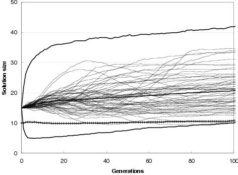
Figure 9.10: Effect of TR recombination transfer limit upon evolution of [left-upper] representation and [left-lower] program size and [right] component expression.
This decoupling characteristic allows program size evolution to follow a different pattern to representation length evolution. Figure 9.10 shows that the number of components transferred or removed during TR recombination has a significant effect upon the evolution of representation length for an initial length of 15 components. This is presumably because (for this initial length) greater transfer lengths allow exploration of a greater number of larger representation lengths without a similar increase in the number of shorter lengths which can be sampled. The trend for program size, by comparison, is far less pronounced. Indeed, it appears that program size is attracted towards a certain level regardless of representation length. This behaviour can also be seen in figure 9.11, in which initial representation length, whilst having a significant effect upon initial program size, has a relatively small effect upon the final average program size within a population. Consequently, for larger initial representation lengths, program size tends to evolve towards smaller solutions. In general, this would seem to be a beneficial behaviour; and certainly favourable to the bloating behaviour found in conventional GP. However, it could conceivably lead to evolution preferring a smaller sub-optimal solution over a larger optimal solution: although this behaviour was not observed in the test problems and recovery from this situation is made more likely given that representation length does not follow a similar trend.
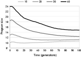
Figure 9.11: Evolution of program size with different initial representation lengths.
21Computational effort is a measure defined by Koza [1992], giving the number of solution evaluations required to achieve a 99% confidence of finding an optimal solution to a problem.
22Note that it is considerably harder to find a solution with no output errors than it is to find a solution with one output error.
23This is akin to the
removal bias cause of bloat seen in tree-based GP.