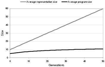
Figure 9.12: Comparing program size growth against forced representation growth in a population of size 100 with no selection pressure, no removal operation and no mutation.
Before attempting to explain why program size evolution follows the pattern described above, this section addresses a related question: Why does the proportion of non-coding components within a representation increase over time? This trend can be seen in both figure 9.924 and figure 9.10. In part, this question can be answered by comparison to Miller's assertion that neutral growth in cartesian GP is due to the exploration of neutral variants within a problem's search space; most of which have more rather than less redundant components than existing program representations [Miller, 2001]. However, a more general answer to this question is that growth in the number of non-coding components is due to variation filtering.
Figure 9.12: Comparing program size growth against forced representation growth in a population of size 100 with no selection pressure, no removal operation and no mutation.
The effect of variation filtering upon neutral growth can be seen in figure 9.12; which shows the pattern of growth in a population which is not undergoing fitness-based selection. Consequently, any problem-specific size information is removed. Again, program size growth is considerably lower than representation size growth, implying that the proportion of un-expressed components in a program representation, on average, increases over time. This effect can be accounted for by a process of variation filtering, where the un-expressed portion of the representation contains those components which have been inserted into the representation but not propagated to the program.
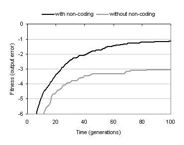
Figure 9.13: Effect of removing non-coding components upon fitness evolution (bs=2).
This un-expressed portion of the program representation constitutes the recessive part of the subsumption hierarchy described in section 9.4.3. Although it would not normally grow at the rate seen in this example, it is interesting to consider whether it has a role other than filtering out components that do not fit into the context of a program. Figure 9.13 shows that when recessive components are removed from representations following program development, fitness evolution is substantially impaired. In fact, in this experiment enzyme GP was not able to evolve any 100% correct solutions when non-coding material was removed. This suggests that recessive components do play an important role in evolution. One of these roles is likely to be maintenance of diversity: making components which are not currently used within programs available for use within future solutions. However, it also seems plausible that recessive components enable evolutionary back-tracking; since if the population were to evolve towards a local optimum, these recessive subsumption hierarchies contain information that could be used as a means of escape to some previous point before the population converged upon the local optimum.
|
|
|
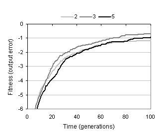
Figure 9.14: Comparing fitness evolution and performance for different numbers of binding sites per component. All functions used are two-input, meaning that recessive binding sites are present for bs > 2.
Figure 9.14 shows the effect of another source of redundancy, recessive binding sites (see section 8.4.1), upon fitness evolution and performance. Whilst the effect is fairly small, there is a statistically significant (U=1255.5, p < .05) performance benefit to having a single recessive binding site for every functional component. However, the benefit becomes insignificant when too many recessive binding sites are used (comparing bs=2 to bs=5: U=914, p=0.2). Again, the benefit to having recessive binding sites probably lies in the extra diversity that they confer. However, too many recessive binding sites presumably interfere with pattern calculation; and can encourage macro-mutation.
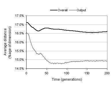
Figure 9.15: Evolution of phenotypic linkage.
The phenotypic linkage of a program is determined by the average Hamming distance between binding sites' functionalities and the functionality shapes of the substrates they bind during development. Phenotypic linkage is a measure of the internal cohesion of a developed program; and therefore a measure of its relative fragility when exposed to evolution.
As figure 9.15 shows, the distance between binding sites and their substrates falls over the course of evolution. This implies that phenotypic linkage increases during evolution. This effect is fairly small for the average distance within the entire program. However, it is more pronounced for the average output distance. This is presumably for two reasons. First, components near the outputs of a program have the most impact upon the program's behaviour and are therefore likely to benefit most from the increased protection from change offered by tighter linkage. Second, variation filtering is more pronounced for the components near the outputs since they have less developmental constraint and are therefore more able to choose substrates which more closely match their binding sites.
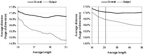
Figure 9.16: Relationship between average phenotypic linkage and representation length [left] during fitness-based evolution and [right] for random solutions. Broken lines indicate common region of representation length between graphs.
However, the effect shown in figure 9.15 is not entirely due to evolution searching for tighter linkage. As figure 9.16 illustrates, tighter linkage is an automatic by-product of larger representation length. This is not surprising, since larger representations offer more choice during development: such that each binding site both has more choice of potential substrates and is more likely to be able to select a given substrate. Given that representation length does, on average, increase during evolution, a proportion of the growth in phenotypic linkage seen in figure 9.15 can be attributed to this increase in representation length. Nevertheless, as figure 9.16 shows, a substantial amount of the growth in phenotypic linkage does appear to be due to evolution searching for tighter linkage. It could even be argued that evolution tends to search longer representations in order to improve phenotypic linkage.
|
|
|
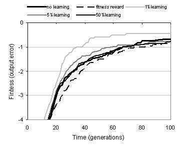
Figure 9.17: Effect of phenotypic linkage learning upon performance. Learning rate refers to percentage change in distance per functionality dimension during Lamarckian reinforcement learning.
Even without taking the effect of representation growth into account, the average increase in phenotypic linkage during the course of a run is not large. This raises the question: can evolutionary search be improved by making an explicit attempt to evolve tighter phenotypic linkage? Two strategies were used to answer this question. The first used an altered fitness function which rewards programs with tighter linkage. The second uses Lamarckian reinforcement learning: whereby following development, binding sites are changed (from the bottom of the program upwards) so that they more closely match the substrates which they have bound. Figure 9.17 shows the effect of these two approaches upon fitness evolution and performance. Where a fitness reward is used, performance is slightly impaired. This suggests that the phenotypic linkage component of the fitness function is interfering with the behavioural component; presumably because programs with tight linkage are not necessarily those with the highest behavioural evolvability. Reinforcement learning, by comparison, can lead to a considerable improvement in evolutionary performance. However, this improvement is dependent upon an appropriate learning rate. If the learning rate is set too high, then there is no improvement in performance. Whilst tighter linkage does both increase the fidelity of development and decrease the disruptiveness of variation operators by encouraging phenotypic building blocks, it must also reduce the scope of search by reducing exploration of new phenotypic building blocks - and hence the number of programs which can be sampled by variation operators. It seems, therefore, that in this case a learning rate of 1% per dimension represents an appropriate balance between phenotypic stability and phenotypic exploration.
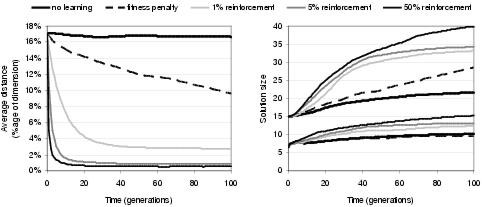
Figure 9.18: Effect of phenotypic linkage learning upon [left] phenotypic linkage, [right-upper] representation length and [right-lower] program size.
Figure 9.18 shows the effect of reinforcement learning upon phenotypic linkage and program size. Not surprisingly, higher levels of reinforcement learning lead to greater phenotypic linkage. However, higher levels of reinforcement learning also lead to larger program size and representation length. Presumably this happens as a consequence of increased phenotypic linkage; suggesting that higher phenotypic stability supports the evolution of larger programs - and that ordinarily it would be more difficult to evolve larger programs25. This observation helps to explain why enzyme GP tends to evolve small programs. Small programs are better replicators than large programs since they have fewer connections between components and are therefore less likely to be disrupted by variation operators. Small programs and their sub-structures are also more likely to be copied by transfer operations.
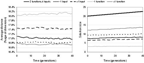
Figure 9.19: Effect of size of function and input terminal sets upon [left] phenotypic linkage and [right] program size (thick black line shows average representation length) for evolution without selective pressure.
Figure 9.19 illustrates that the size of the function and terminal sets affect the behaviour of evolution even when a population is not exposed to selective pressure; indicating that program evolution is biased by the constitution of the activity set in a way which is independent of the problem's search space. This is one of the less desirable properties resulting from the use of functionality as an implementation of implicit context. Specifically, increasing numbers of functions and decreasing numbers of input terminals both lead to larger program size and higher phenotypic linkage. In part, this happens due to an implicit bias towards expressing preferences for input terminals over functional activities within random functionalities. Each function and input terminal activity is allocated one dimension in functionality space. However, whereas there are many copies of each functional component within a representation, there is only one instance of each input terminal. Consequently, there is a disproportionately high likelihood of a random functionality expressing a strong preference for an input terminal activity: although during selective evolution (where functionalities do not remain random) this is unlikely to be a problem unless a strong sub-optimal solution has a high proportion of input terminals close to its outputs. Nevertheless, this implicit bias may be another reason why enzyme GP tends to evolve short programs; and, as figure 9.19 shows, is a behaviour which can be altered by changing the ratio between input terminal activities and functional activities.
A further explanation for the effect of function set size upon program size and phenotypic linkage may lie in the degree to which a function set can express large solutions. A component's functionality describes an expected profile of the functions which will occur in the sub-program of which it is the root. If a lot of different functions are used in a program, then functionality has a relatively large amount of detail with which to describe a sub-program. If there are fewer functions, then functionality has less detail with which to describe a sub-program and consequently less scope with which to distinguish between components. Accordingly, programs with fewer functions may have a tendency to display less internal cohesion and be more sensitive to variation, tending towards smaller sizes in order to gain sufficient replication accuracy.
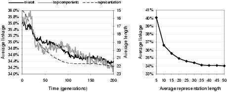
Figure 9.20: Average genetic linkage between components as a percentage of representation length. [Left] Evolution of genetic linkage for all components (`overall') and for components bound to outputs (`top components'), showing average representation length. [Right] Relationship between representation length and average genetic linkage without evolution.
Figure 9.20 shows the pattern of genetic linkage evolution within enzyme GP. As with phenotypic linkage, larger representation lengths automatically generate tighter genetic linkage. This occurs because larger representations tend to have lower levels of component expression, implying that the expressed components can on average cover a smaller portion of the representation. Compensating for this trend, genetic linkage does appear to evolve in enzyme GP, but at a very low rate (a few tenths of a per cent over the course of two hundred generations). The genetic linkage learning rate is slightly higher for components located proximal to the program outputs. Again, this would be expected given the greater value of building block formation nearer to the program outputs. In figure 9.20, the output linkage continues to improve following the convergence of representation length: though given the variance suggested by the noisy plot, this may not be a representative trend. In general, these results suggest that genetic linkage is not encouraged by enzyme GP. Accordingly, it might be interesting to investigate the merit of genetic linkage reinforcement considering the apparent benefit of phenotypic linkage reinforcement. Whilst it might not be possible to improve the genetic linkage between all pairs of interacting components, it certainly seems possible that genetic linkage could be improved on average, for components near program outputs, or for the most strongly interacting components in a program.
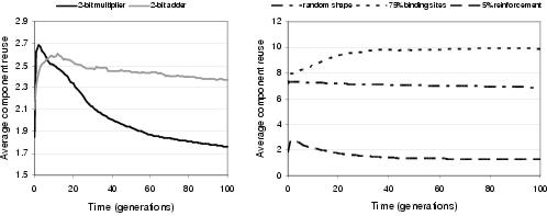
Figure 9.21: [Left] Evolution of functional component reuse for two-bit multipliers and adders. [Right] Some factors which affect component reuse during the evolution of two-bit multipliers.
Component reuse is the number of times a single component instance is bound during development. Accordingly, average component reuse measures how many times, on average, sub-expressions are reused within programs. Figure 9.21 shows how the average functional26 component reuse changes during the course of evolution. These graphs display a number of trends: (i) the pattern of reuse is problem independent; (ii) reuse generally falls during evolution; and (iii) components are typically used more than once during program development. Implicit context is expected to promote a degree of component reuse; since, according to the definition of implicit context, behavioural reuse should require component reuse. It is therefore to be expected that the degree of reuse will depend upon the problem's search space - and presumably for both of these problems, behavioural reuse becomes less appropriate as search approaches the optimal program behaviour. Figure 9.21 also shows that reuse is affected by both reinforcement learning and the manner in which component shape is derived. For reinforcement learning, it is more likely that component reuse will reflect behavioural reuse, given that distances between components are likely to be smaller. This tends to suggest that without reinforcement learning, there is more reuse than is strictly necessary to express solutions. Where shape is generated randomly or heavily biased towards binding sites, reuse rises considerably. This reflects a decreased bias towards input terminal components, making it more likely that functional components will be bound during development.
These results indicate that evolution can take place using a wide range of degrees of component reuse. However, no attempt has been made to measure the relationship, if any, between reuse and evolutionary performance. Given the current debate amongst evolutionary biologists over the relative merits of compartmentalisation and pleiotropy, this would be an interesting investigation for future work.
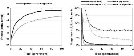
Figure 9.22: [Left] Fitness evolution and [right] recombinative behaviour of development strategies.
Two different development strategies were outlined in section 8.5. Top-down development constructs a program from the outputs to the inputs, whereas strongest-first development constructs a program from the most strongly interacting components to the least strongly interacting components. Accordingly: (i) strongest-first development leads to higher average phenotypic linkage; (ii) top-down development leads to higher phenotypic linkage nearer to the program outputs; and (iii) strongest-first development is able to construct connections between components which do not contribute to the program outputs. Figures 9.22 and 9.23 show the consequences of these behaviours upon evolutionary performance, recombination, and development time. Top-down development supports better evolutionary search than strongest-first development. Figure 9.22 suggests that the relatively poor performance of strongest-first development may be due, at least in part, to lower recombinative success and lower neutral exploration through crossover. It is not entirely clear why this is the case. However, it might be speculated that this is due to lower phenotypic linkage between components near the program outputs; leading to lower correspondence between the expected behaviour and the actual behaviour of these behaviourally important components. This, in turn, could lead variation operators to more easily disrupt the behaviour at the program outputs.

Figure 9.23: Relationship between development time and solution lengths.
Figure 9.23 shows that top-down development also offers better time complexity than strongest-first development. This follows from point (iii) above. For top-down development, the fact that program size growth is a lot lower than representation length growth means that development time only rises at a near linear rate with respect to representation length; despite the fact that the development process has above-linear time complexity with respect to program size (see rightmost graph in figure 9.23). For strongest-first development, connections are made which are not part of the developed program; and since the number of connections made rises in line with representation length growth, the rate of development time growth is much higher than linear with respect to representation length growth.
It seems clear that, in principle at least, meaningful variation filtering is a key ingredient in the hunt for an evolvable representation. Perhaps the most persuasive evidence that implicit context leads to meaningful variation filtering is that search performance (figure 9.2) and the relative capacity for recombination to generate fitter children (figure 9.6) both decrease considerably when implicit context is replaced with a form of indirect context. Hence, it follows that these beneficial behaviours are a consequence of program components choosing their interactions according to behavioural descriptions of other components rather than arbitrary patterns. To a lesser extent, this argument is also supported by performance comparison between enzyme GP and cartesian GP (section 9.2); although this comparison is made unreliable by the many other differences between the two methods.
The argument that implicit context representations react in a meaningful way to change is also supported by the recombinative behaviours outlined in section 9.4.3 which occur as a result of the addition and removal of components. For each of these behaviours - subsumption, insertion, and removal - the child program `attempts' to preserve the behaviours of the parent despite changes to the program's representation: yet still allows change to occur. Nevertheless, there has been no quantitative study of how often, and how effectively, these behaviours occur during program evolution; and whilst they are seen to occur frequently, they are rarely as pure as in these examples. Furthermore, many of the behaviours which are seen during evolution do not have such evidently beneficial characteristics. Therefore, whilst implicit context does lead to improved variation filtering behaviours when compared to indirect context, it seems fair to contend that this does not happen for all variation events. However, this is generally the nature of evolutionary search.
This is an extension to the previous point. As well as improving the capacity for a representation to receive new components, implicit context also improves the likelihood of components maintaining their meaning when transferred between programs; and hence the capacity for a population to carry out co-operative evolution. This follows from the observation that recombination between pairs of existing representations leads to better evolutionary performance than headless chicken recombination between existing representations and randomly constructed representations (figure 9.5). Presumably this performance advantage is due to relatively fit program fragments being transferred between existing representations. Nevertheless, whilst there is a significant difference between the performance of recombination and headless chicken recombination, the performance of headless chicken recombination is still relatively high. That a macro-mutation operator can apparently carry out useful search supports the notion that implicit context representation improves response to variation. However, it also gives some concern that response to variation is dominant over transfer of information in generating recombinative performance. Consequently, in future work it might be interesting to take a closer look at how well information is transferred between programs and whether there are mechanisms which might improve the fidelity of information transfer. Genetic linkage reinforcement may be one such mechanism; since interacting groups of components are more likely to be transferred as a unit if they are located proximal in the representation. Without genetic linkage between components, there is some danger that transfer operations are more likely to transfer a group of small, non-interacting, program fragments which may either lose their behaviours or disrupt multiple sub-structures within the recipient program. Whilst some authors [e.g. Keijzer et al. 2001] believe that it is beneficial to change a program at multiple locations during recombination owing to increased search potential, it also seems that this sort of operation is more likely to disrupt the evolved behaviour of the program and lead to inviable offspring.
This follows from the previous two points which show that functionality leads to the kinds of behaviours that would be expected from a meaningful implementation of implicit context. However, it appears that functionality is only meaningful when its derivation reflects an appropriate balance between a component's activity and its binding sites (figure 9.3). Otherwise, functionality fails to capture a sufficient description of a component's behaviour: either by not sufficiently describing how a component interacts with other components, or by not sufficiently describing the components it interacts with.
Despite its ability to describe implicit context, and the ease with which it can be calculated, functionality is not an ideal implementation of implicit context. Functionality is limited to describing contexts in terms of a functional profile. It can not describe the ordering or interactions between the functions in this profile. Whilst this is evidently sufficient to describe solutions to the problems used in this chapter, it apparently struggles to describe the kind of structural reuse seen in solutions to parity problems (section 9.2), and it is conceivable that it is not sufficient to describe all types of structure. Consequently, an important future avenue of research would be to investigate the applicability of functionality and, if necessary, consider other implementations of implicit context.
Whilst, in some circumstances, enzyme GP structures experience a degree of growth; enzyme GP does not experience conventional GP bloating behaviour (figure 9.9). Recall from section 6.4 that there are a number of hypothesised causes of bloat within tree-based GP: replication accuracy, removal bias, search space bias, and operator bias. The replication accuracy theory contends that bloat is needed to protect programs from the disruptive effects of recombination. It seems that whilst the recombination operators of enzyme GP do not always carry out meaningful behaviour, TR recombination in enzyme GP is less disruptive than sub-tree crossover in tree-based GP. Partly this is a result of variation filtering at the representation level. However, disruption is also reduced by the decoupling between transfer and remove operations. Whereas in conventional GP, one group of components always replace another; in enzyme GP transfer does not physically replace components, and remove operations operate independently to transfer operations. Furthermore, as with linear GP (see section 7.4.1), non-coding components within enzyme GP representations are able to provide a structural protection role which can, in principle, increase reproductive fidelity without the need for the kind of global protection behaviour provided by bloating in tree-based GP.
Removal bias can still be caused by the disparity between the success rate of transfer and remove operators; but does not have the potential to drive bloat at anything like the levels seen in tree-based GP. Search space bias is a property of the problem domain rather than the search process, so presumably is still a factor in enzyme GP. There is no operator imbalance in enzyme GP, since recombination - at least mechanistically - has a size neutral effect. In summary, it seems that the lack of bloat in enzyme GP can in part be explained by a lessening of the behaviours hypothesised to cause bloat in conventional GP. However, it seems that the remaining behaviours, particularly search space bias, should have the capacity to drive a certain amount of size growth: yet this growth is not seen in practice.
This occurs because components present in the representation need not be expressed in the program. However, the representation length does place an upper limit upon the program size, even after component reuse has been taken into account. The advantage of this decoupling is that program size evolution is not directly linked to the action of the recombination operators and is therefore free to vary within the upper bound set by the representation length. In practice it appears that evolution is biased towards searching smaller program sizes: which, from a practical viewpoint, is advantageous since it leads to small, efficient solutions. It also helps to explain why representation length does not bloat, since there is little search pressure towards higher upper limits on program size.
There appear to be two reasons for this behaviour (section 9.7.2). First, functionalities with a disproportionately high degree of input terminal activities are over-represented in functionality space; giving functionality space an implicit bias towards short solutions. This bias is particularly apparent when the activity set contains many input activities and few functional activities (figure 9.19). Nevertheless, the bias only applies to random functionalities; and consequently dissipates as functionalities become non-random during the course of evolution. Second, small programs presumably have higher replication fidelity since they have less internal connections to be disrupted when exposed to variation operators and, having shorter defining component sequences, are more likely to be propagated during transfer operations.
In part, the trend towards smaller program size compensates for the higher time complexity resulting from the development process (figure 9.23). It also leads to lower space complexity. However, there is some danger that enzyme GP will find it harder to solve problems with large solutions; particularly if sub-optimal solutions are short. Some useful directions for further research will be to look at ways of removing functionality bias, possibly by selecting more representative initial generation functionalities, and ways of reducing the complexity of development. Perhaps the most obvious way of reducing complexity would be to allow recurrent solutions; since most of the development time is involved with preventing recurrency.
This follows from the observation that when redundant components are removed from program representations following development, evolutionary search is substantially impaired (figure 9.13). The beneficial effect of non-coding components could either be due to a structural or functional role. Although a structural role can not be discounted, it seems relatively difficult for non-coding components to carry out a structural protection role in enzyme GP given that (i) there is little genetic linkage between interacting components, and therefore little scope for the construction of linear sequences of non-coding components between coding sequences; (ii) non-coding components do not necessarily remain non-coding following transfer, and therefore do not substantially decrease recombinative disruption; and (iii) there is relatively little scope for the construction of syntactic introns. However, there are good reasons to believe that redundancy provides a beneficial effect through its functional role. Considering that program size tends towards small solutions, it would be easy for a population to lose functional diversity if it were not for the substantial proportion of non-coding components found within representations. Furthermore, it seems that this redundancy must be organised in the form of a subsumption hierarchy (section 9.4.3); where the components at the top of the hierarchy may play a key role in enabling back-tracking behaviours in response to disruptive variation events. This apparently beneficial functional role of redundancy also agrees with the findings of much of the research reviewed in section 7.4.3.
A reinforcement learning rate of 1% of the difference between a binding site and the shape of its bound component leads to a 50% improvement in success rate and a significant reduction in the average number of generations required to evolve a two-bit multiplier (figure 9.17). Presumably this is due to the stabilising effect that reinforcement learning has upon the building blocks of evolving programs. Given that interactions are reinforced following each variation event, reinforcement learning will give most stability to those building blocks which have remained in the same program throughout a number of variation events or have passed through a number of programs via transfer operations. Therefore, reinforcement learning implicitly strengthens those building blocks which have a high effective fitness; and in effect increases their effective fitness over time by making them easier to propagate between programs. The benefits of Lamarckian reinforcement learning within enzyme GP mirrors its benefits within other GP systems [Teller, 1999,Downing, 2001]. The trade-off between exploration and exploitation in choosing an appropriate learning rate in enzyme GP also mirrors the balance between insufficient learning and over-learning when choosing a learning rate for the neural network back-propagation algorithm.
24Ignoring uniform crossover, which is assumed not to have a significant effect upon size evolution.
25This does not suggest that large programs are impossible to evolve, just that smaller programs are more likely to be propagated by the evolutionary mechanism; and therefore preferred over larger programs with equivalent functionality.
26Input terminal component reuse is ignored since there is only one instance of each input terminal and therefore an un-representative amount of reuse of these components.