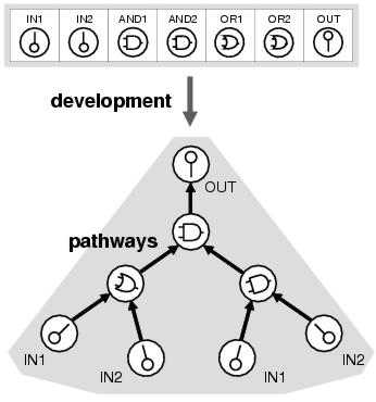
Figure 8.1: A program in enzyme GP is represented by a linear genome which is mapped into a program via a process analogous to the development of metabolic pathways.
Enzyme genetic programming [Lones and Tyrrell, 2001c,Lones and Tyrrell, 2001b,Lones and Tyrrell, 2001a,Lones and Tyrrell, 2002b,Lones and Tyrrell, 2002a,Lones and Tyrrell, 2003b,Lones and Tyrrell, 2003a] is a genetic programming system that uses a program representation modelled upon the organisation and behaviour of biological enzyme systems. This chapter introduces enzyme GP and discusses the motivation behind the approach.
A metabolic network is a group of enzymes which interact through product-substrate sharing to achieve some form of computation. In a sense, a metabolic network is a program where the enzymes are the functional units and the interactions between enzymes are the flow of execution. Enzyme GP represents programs as structures akin to metabolic networks. These structures are composed of simple computational elements modelled upon enzymes. The elements available to a program are recorded as analogues of genes in an artificial genome. These genomes are then evolved with the aim of optimising both the function and connectivity of the elements they contain. The mapping between genome and program is conceptually depicted in figure 8.1.
Figure 8.1: A program in enzyme GP is represented by a linear genome which is mapped into a program via a process analogous to the development of metabolic pathways.
From a non-biological perspective, enzyme GP represents a program as a collection of components where each component carries out a function and interacts with other components according to its own locally-defined interaction preferences. A program component is a terminal or function instance wrapped in an interface which determines both how the component appears to other components and, if the component requires input, which components it would like to receive input from.
Program evolution within GP is a consequence of processes of change, such as mutation and crossover, acting upon the program's representation. In the absence of intelligent variation operators, program evolvability is determined by the ability of the representation to respond to change: in particular its ability to promote meaningful change whilst preventing the expression of inappropriate change. Chapter 6 recounts how the standard GP program representation, the parse tree, fails to support recombination - a conceptually meaningful evolutionary behaviour - whilst promoting program size bloat, a generally inappropriate behaviour. Parse trees lack evolvability because they have no nascent ability to filter change; and even when the representation languages of particular problem domains enable `emergent' filtering mechanisms, such as the global resistance to semantic change offered by syntactic introns, the resulting bloating behaviour is inappropriate.
Chapter 7 reviews ways in which potential sources of evolvability can be introduced to the representations of genetic programming and other evolutionary algorithms, and how this approach generally leads to improved evolutionary behaviours and computational performance. Many of these sources of evolvability were identified by looking at the representations of biological organisms, and this seems to vindicate the notion that biological modelling can be used to improve the behaviour and performance of evolutionary computation - and forms part of the motivation for the development of enzyme genetic programming. The program representation used by enzyme GP is modelled both upon the way in which the function of biochemical pathways emerges from the sum of the behaviours of individual proteins and enzymes, and upon the way in which these systems respond to genetic change. Enzyme GP possesses many of the characteristics identified within the previous chapter as being sources of evolvability: including positional independence, functional and structural redundancy, neutrality, and implicit reuse.
The role of context within program representation is perhaps central to an understanding of enzyme GP and how it differs from other genetic programming approaches. According to the definition given in Section 6.3, a program component's context is determined by where it receives its inputs from: since this determines the arguments to which its function will be applied and therefore its outputs and hence its role within the program.
Within a parse tree, the context of a program component is determined by its position within the structure. For the remainder of this manuscript, this form of context is called explicit context, reflecting the fact that a component's context is recorded explicitly by its position within the representation relative to other components. Other GP approaches which use explicit context representations include linear GP [e.g. Nordin, 1994] and grammatical evolution [e.g. Ryan et al. 1998]. Explicit context representations have two properties which limit their ability to be evolved. The first, that a component's context is determined by position, that crossover operators do not preserve this position, and that therefore contextual information is easily lost, has already been discussed at length. Second, explicit context usually enforces a one-to-one mapping between representation and program, such that changes to the representation lead directly to changes within the program. The variation operators therefore act directly upon the program, implying that evolution is determined solely by processes of variation and selection. The representation, by comparison, has no dynamic role to play within the evolutionary process.
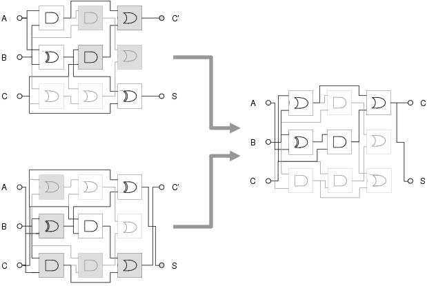
Figure 8.2: Recombination can cause loss of context when indirect context is used. A cartesian GP circuit is recombined with a flipped version of itself, but due to the same components occupying different locations in the two circuits, context (and consequently behaviour) is not preserved in the recombined circuit. Recombined parts are shaded grey.
In some other GP representations [e.g. Poli, 1997, Miller and Thomson, 2000], connections between components are specified using indirection. Typically each component is assigned a reference (which may be a location, a number or an arbitrary code) and other components specify their input connections using these references. A good example of this is Cartesian GP [Miller and Thomson, 2000], where components are assigned to locations in a cartesian co-ordinate system and input connections are expressed in terms of the co-ordinates of components they wish to receive inputs from. Context within these representations is specified indirectly, hence this form of context is termed indirect context.
Indirect context representations support a number of interesting evolutionary behaviours. Perhaps most significantly, a component only becomes active in a program if another component expresses a connection to it. Otherwise it is recessive. This has some important implications. If a new component is added to the representation during recombination, it will only become active in the program if its reference is addressed by an existing component or it is an output node. This effect is termed variation filtering, since the representation only expresses certain variation events in the program whilst filtering out others.
Indirect context representations usually assign references arbitrarily: such that there is no correlation between component reference and component behaviour. Indirect context, therefore, does not declare any behavioural information. Consequently, it expresses no real meaning other than the connectivity of the current program. This leads to similar problems to those seen with explicit context representations. Most significantly, indirect context has no meaning between different programs since components with different behaviours can have the same reference and components with the same behaviour can have different references in different programs. This implies that recombination is unlikely to preserve context (see figure 8.2). Furthermore, if a component's input connection is mutated, there will be no correlation between the degree of mutation and the degree of change to the component's input context: meaning that the component's context cannot be varied gradually, unless by accident.
However, it is conceivable that the population might be able to evolve a correlation between component reference and component behaviour over the course of time, especially as the population becomes more homogenous. In this sense, the meaning of indirect context is evolvable. Furthermore, indirect context representations support both structural and functional modes of redundancy in addition to a capacity for implicit reuse.
By comparison to the explicit and indirect contexts used by GP, biology expresses component interactions with what could be called implicit context. With implicit context, a component's context is declared implicitly within the component's definition rather than being imposed by external factors such as its relative position within a representation. For example, the behaviour of a bio-chemical is dependent upon its physical shape and chemical properties. Enzymes, which conceptually receive their input in the form of bio-chemicals, express their preference for these inputs by the shape and chemical properties of their binding sites. Since the bio-chemicals that they bind have physical shape and chemical properties complementary to the binding sites, these binding sites are implicitly describing the enzyme's context in terms of the behaviour of the substrates they expect to bind.
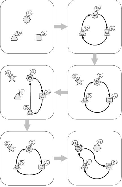
Figure 8.3: Evolution of an abstract implicit context system. [top-left] The system comprises three components. [top-right] The system self-organises according to each component's implicit context. [middle-right] A newly added component is not expressed because it does not match the system's existing contexts. [middle-left] A new component subsumes the role of an existing component. [bottom-left] The system backtracks to a previous state when a new component is lost. [bottom-right] Mutation leads to expression of a recessive component.
Figure 8.3 illustrates an example of an abstract system whose behaviour and evolution is determined by implicit context. The system is represented by three components: each of which has a shape, which identifies it to other components; and an implicit context, which declares the shape of the component it would prefer to interact with. If the system is allowed to develop, interactions occur according to the implicit contexts declared by each component; whereby each component attempts to interact with a component whose shape most closely matches its own implicit context. In essence, the system self-organises according to the properties of the components from which it is comprised. Because of this property of self-organisation, there is no external requirement for a component to be expressed in the developed system. In the example, a component is added to the representation which does not match any of the implicit contexts defined by the existing components and is consequently not `expressed' in the developed structure of the system. Conversely, if a component is added to the representation which has a better match with one of the existing implicit contexts of the system, then it does become expressed in the system.
This is another example of a variation filtering process of the kind seen where an indirect context representation is used. In an indirect context representation, the lack of correlation between indirect context and behaviour causes variation filtering to be an arbitrary process. In an implicit context representation, by comparison, variation filtering is a process which filters out change which does not fit into the current system context whilst promoting change which improves the internal cohesion of the system. From an evolutionary perspective, this would seem like a useful function since it tends to preserve the existing evolved behaviour of the system by lessening the impact of change and without actually preventing change to the representation.
The bottom two panes in figure 8.3 show the benefits of recessive components within an implicit context representation. In the first of these, a component which was added to the system has now been lost; but because the added component had only subsumed the role of an earlier component, rather than replacing it, the earlier component is able to resume its role. This demonstrates a capacity for backtracking, showing how functional redundancy can reduce the impact of the loss of a component upon the behaviour of the system. In fact, this is another example of variation filtering, but filtering the effect of removing a component rather than the effect of adding a component. The final pane of figure 8.3 shows that recessive components are also able to undergo evolution. In this case, the mutation of a recessive component allows it to fit into the context of the system and become expressed.
Implicit context does not seem like an obvious approach to representing programs, yet its pervasiveness in biology and the behaviours described above suggest that it is a good way of representing an evolving system. Indeed, implicit context representation seems to fulfill at least the first of Kirschner and Gerhart's principles of evolvability: the capacity to reduce the potential lethality of mutations - which it achieves through the variation filtering process described above, making it less likely that change to a representation will result in substantial change to the entity that it represents. This in turn makes it more likely that Kirschner and Gerhart's second principle will be met: a capacity to reduce the number of mutations needed to produce phenotypically novel traits; since there is more chance of the entity surviving a series of changes. Moreover, the presence of functional redundancy brings with it the potential modes of evolution described in sections 5.2.1 and 7.4.3; each of which tend to increase the explorative potential of evolution and hence the likelihood of a series of changes leading to an improved entity.
It is hoped that implicit context can be used to introduce variation filtering to program representations, leading to an improvement in the behaviour and success rate of conventional GP variation operators, and in particular enabling meaningful recombination. However, there are certain pre-conditions for implicit context to be able to enable useful variation filtering. These were originally identified in Lones and Tyrrell [2002a] and concern the relationship between implied context (the context declared in the representation) and actual context (the context which occurs in the program). Precision is the generality of the implied context: the degree to which it suggests an actual context. If implicit context is too general, then the behaviour of the program will not be obvious from the representation, making the mapping between representation and program unstable and therefore easily disrupted by the application of variation operators. In turn, this will make meaningful recombination unlikely. Related to precision is the issue of specificity: how well an implied context is able to identify an actual context. If a component's implied context is too unspecific, it is likely to form different actual contexts within different programs, meaning that variation filtering will tend to carry out arbitrary behaviours. Finally, there is the issue of accuracy: the ability of implicit context to match actual context given the availability of components within the representation and any constraints upon connections between components that are placed upon the behaviour of the program. Given that these limitations are unavoidable, there is little that implicit context can do to overcome them. Nevertheless, it is important that when the preferred context is not available, the implied context should match the nearest available actual context. In turn, this requires that a distance metric can be defined between implied and actual contexts, such that the greater the distance between contexts, the greater is the difference in component behaviour.
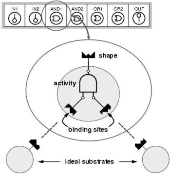
Figure 8.4: Enzyme model. A program component consists of a shape, an activity and a set of binding sites. Shape describes how the enzyme is seen by other program components. The shape of a binding site determines which component (or `substrate') will be bound at a particular input.
The enzyme GP implementation of implicit context is modelled upon biological systems in which the behavioural context of a component is both described and determined by its shape. As depicted in figure 8.4, program components in enzyme GP are loosely modelled upon biological enzymes. Each program component has a shape. This describes the behaviour of the component and also functions as an identifier which can be referred to by other components. Most program components also have a set of binding sites. Each binding site has a shape and this shape identifies the component it would expect to bind during a development process. Accordingly, shape determines where each component will be bound: giving its expected context within a developed program.
Each program component also has an activity. This activity is either a function, an input terminal, or an output terminal; and determines what the program component will do within a developed program. Only components with functional and output terminal activities have binding sites. Following development, the function or output terminal's input(s) will be provided by the output of the components which are bound to the binding sites. Input terminal components provide program inputs at their outputs.
A shape is not just an identifier. Shape also describes the behaviour of a program component. It would be insufficient for shape to merely express the activity of a program component since there will in general be many instances of only a few different functions and terminals within each program. Nevertheless, each of these instances will be carrying out a different role within each program. The aim of shape within enzyme GP is to capture this role.
The role of a program component depends not only upon itself and the activity it carries out but also upon the components it interacts with and the activities they carry out. In particular, the outputs of a functional activity depends upon its inputs, and this depends upon the components it receives its inputs from, whose outputs, in turn, depend upon the components they receive their inputs from, and so on. In fact, for parse trees, the outputs of a program component - its behaviour - are dependent upon all the activities of all the components which occur below it within a program. These activities are the information which a shape attempts to capture.
In essence, a program component's shape describes a profile of the activities which are expected to occur within the sub-tree of which the component is the root. This profile is called a functionality and is derived solely from the component's activity and binding sites. Information regarding the activities at and below the binding sites is inferred from the shapes of the binding sites: since these shapes give the functionalities of the components which are expected to be bound during development.
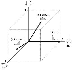
Figure 8.5: Functionality space for function set {AND, OR} and terminal set {IN1} showing example functionalities. Two-dimensional vector plots of functionalities, such as those shown in this figure, are used for illustrative purposes throughout this chapter.
Formally, a functionality is a vector which describes the component's position within
an activity reference space. This reference space has one dimension of unit length for
each member of the GP function and terminal sets (see figure
8.5 for an example). The functionality, F, of a program
component is a weighted vector sum of the functionality of its activity and the
functionality of its binding sites, defined as follows:
| (8.1) |
where inputbias is a constant that biases the functionality towards either the
component's activity or the component's binding sites; F(activity), the functionality
of the component's activity, is a unit vector situated in the dimension corresponding
to the enzyme's function; and F(binding_sites), the functionality of the component's
binding sites, is defined:
| (8.2) |
i.e. the average of the functionalities corresponding to its binding sites weighted by the strength (a value between 0 and 1) of each binding site. Strengths are used to determine which binding sites are active when there are more binding sites than there are inputs to the activity. For instance, if a component has a two-input activity and three binding sites, only the two binding sites with the highest strengths will bind components during development.
An illustrative example of equations 8.1 and 8.2 is shown in figure 8.6, showing how a derived functionality captures the activity profile of a component's expected sub-tree.
In effect, a component's functionality declares an expected activity profile of the components that occur in the program fragment of which it is the root, weighted by depth and biased by the strength of binding sites. Functionality space itself is continuous and the distance between functionalities is calculated using vector subtraction. This reflects the difference between their activity profiles, meeting the requirement (outlined in the previous section) that the greater the distance between contexts, the greater is the difference in component behaviour.
However, the functionality approach has two inherent limitations. First, a functionality only gives a profile of the activities within an expected sub-tree. It does not describe where they occur within the sub-tree and how they are inter-connected. Second, a functionality only gives an expected profile. During development, it may not be possible for a component to bind the exact components described by its binding sites: either because they are not available within the program's representation or because there are constraints upon development (see following section).
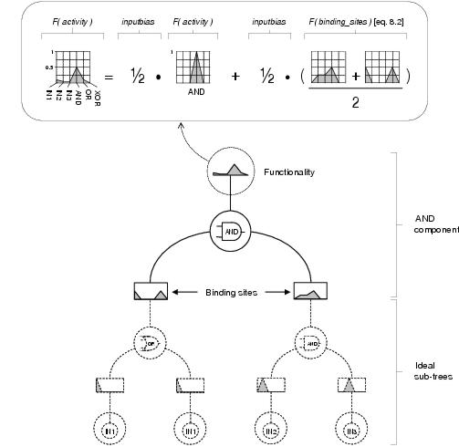
Figure 8.6: Derivation of functionality. An AND component's functionality is derived from the functionality of the AND function and the functionalities declared by its binding sites using equations 8.1 and 8.2 with inputbias = [1/2] and assuming both binding sites have a strength of 1. The component's functionality captures a profile of the function and terminal content, weighted by depth, of itself and its ideal subtrees i.e. a high proportion of AND functions, a significant proportion of OR functions and IN1 terminals, a low proportion of IN2 and IN3 terminals, and no XOR content.
An enzyme GP program consists of three types of component: input terminals, functional elements, and output terminals. A program's representation is the enzyme GP analogue of a biological genome: stored as a linear array of program components; the format of which is shown in figure 8.7. This program representation records the components which are available to the program and that may be expressed within the program following a process of development.
The objective of the development process is to map the program representation into a program in such a way that each active input of each active component will be connected to the output of the component for whose shape its corresponding binding site has the highest specificity i.e. the shortest distance between functionalities. Two different development processes have been used in this research, although others are possible. The first, which could be called top-down development, begins with expression of the output terminals, which then choose substrates whose shapes are most similar to the shapes of their strongest binding sites. These substrates are now considered expressed and, if they require inputs, attempt to satisfy them by binding their own substrates. This process continues in hierarchical fashion until all expressed program components have satisfied all of their inputs. This development process is illustrated in figure 8.8 by way of an example.
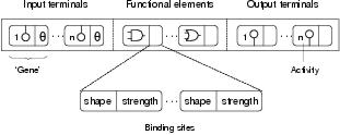
Figure 8.7: Format of a program representation, showing its division into input terminal, functional element and output terminal components. Every program representation contains a full set of input and output terminals components. Note that input terminal components do not have binding sites, for they receive no input from other components. Also note that component shapes are generated dynamically and do not therefore appear in the program representation.
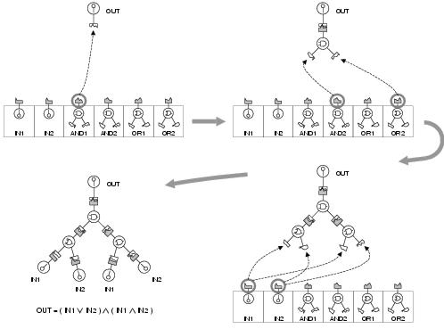
Figure 8.8: Top-down development of a simple Boolean expression. The first component to be expressed is the output terminal receptor. This then binds as a substrate the component whose shape is most similar to its binding site; the AND1 component. The AND1 component now chooses its own substrates and the process of substrate binding continues until the inputs of all expressed components have been satisfied. Note that OR1 is never expressed and that IN1 and IN2 are both bound twice.
The alternative development process involves transforming the program representation into a network random key representation of the kind described by Rothlauf and Goldberg [2002]. In essence, this means that connections between components - and hence the components involved in the connections - are expressed in order of strength: where the strength is the vector difference between a binding site and a shape. The strongest connections are expressed first and connections continue to be expressed until a complete structure has developed where every expressed component has all its inputs satisfied. This development process is called strongest-first development.
For both development processes, each output terminal is expressed exactly once, whilst input terminals and functional elements can be expressed once or not at all. Where more than one component chooses the same substrate, the output of the substrate is shared between them: introducing a capacity for implicit re-use as described in section 7.3.2. In problem domains where there are no constraints on component interaction, both of these development processes should produce identical mappings between program representation and program - except that strongest-first development might lead to extra expressed components and connections which do not contribute to the program outputs by virtue of output terminal components being able to choose inputs internal to expressed structures (see figure 8.9).
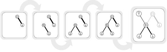
Figure 8.9: An example of strongest-first development. Line thickness shows the relative strength of a bond. Note that the components coloured grey in the developed circuit do not contribute to the circuit's output even though they are expressed during development.
However, where the problem domain introduces constraints on development, different development processes can lead to different mappings. For the problem domains used in this research, programs are constrained to have tree-structures and therefore must contain no cycles. This constraint is handled within both development processes by checking for the presence of cycles before a new connection is made. If a connection to a substrate would result in a cycle, then an alternative (less preferred) connection must be made. Where cycle prevention is used, development becomes sensitive to the order in which connections are expressed. During top-down development, cycles are prevented by stopping components from making connections to those components which already appear above them in the program tree. The further down a component appears in a program, the higher is the degree of constraint upon which components it can choose to bind and therefore the lower is the likely match between the components it wishes to bind and the components it actually binds. Accordingly, linkage will tend to be relatively high near the top of developed programs and relatively low near the bottom of developed programs. For strongest-first development, by comparison, high linkage connections would be distributed around the program. Because this development process promotes the expression of high linkage connections, it would also be expected that connections would be stronger on average than those in programs resulting from top-down development.
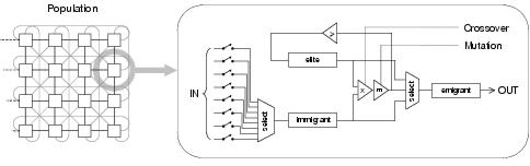
Figure 8.10: Structure of the network genetic algorithm, showing the organisation of the population and the processing which occurs in each cell of the population during each generation.
Evolution of program representations occurs within the framework of a diffusion model distributed genetic algorithm called the Network GA [Lones, 1999] (depicted in figure 8.10). The population is organised into a spatially-distributed network of cells, each of which carries out an evolution strategy upon local state and inputs from surrounding cells. The network topology determines the processing behaviour of the population. For all experiments reported in this thesis, the network is a two dimensional edge-connected matrix (toroidal). A cell's evolution strategy selects the fittest individual from the emigrants of those cells designated as inputs by the network. This immigrant then undergoes recombination with the local elite; the fittest individual created so far within this cell. If the fittest child is fitter than the elite, then the elite is replaced with this child. The cell's emigrant is the fittest individual out of the parents and the children. By implementing elitism, the algorithm retains fit solutions. By making this elitism local to each cell, diversity is preserved and new solutions are encouraged. Diversity is also encouraged by the spatially-distributed structure of the population and the accurate sampling enabled by local selection. Whilst each cell contains three individuals, only the elite is considered resident and only the children are evaluated during each generation. The network GA was chosen both for its diversity-preserving behaviour - which allows the effects of neutral evolution to be more easily studied - and more generally for its use of a spatially-distributed population structure, which allows evolution to be easily visualised.
At the start of an evolutionary run, the population is filled with randomly generated program representations: each of which has a preset number of input and output terminal components and a randomly chosen assortment of functional components. The number of functional components within a program representation is initially bounded but is allowed to vary freely during evolution. The activities of functional components are chosen non-deterministically. The dimensions of binding site functionalities are also chosen randomly, though not necessarily from a uniform distribution.
Enzyme GP uses both mutation and recombination (both separately and in concert) to generate new program representations from existing program representations. Mutation is able to target both activities and binding sites. Activity mutation is only applied to components with functional roles and works by replacing the current function with a new function chosen at random from the problem's function set. Binding site mutation targets each dimension of the binding site's functionality with equal probability; replacing the current value with a new value chosen at random according to the same probability distribution that was used during initialisation.
The experiments reported in the following chapter use two different kinds of recombination. Uniform crossover intentionally generalises the uniform crossover operator used by genetic algorithms and loosely models biological recombination. Uniform crossover is a two-stage process of gene recombination followed by gene shuffling. Gene recombination resembles meiosis, the biological process whereby maternal and paternal DNA is recombined to produce germ cells, and involves selecting and recombining a number of pairs of similar components from two parent program representations. Pairs of components are selected according to the similarity of their shapes and standard GA uniform crossover is used to recombine their binding sites. Gene shuffling then divides the recombined components uniformly between two child program representations. Figure 8.11 illustrates the resemblance between enzyme GP uniform crossover and meiosis.
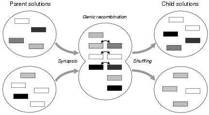
Figure 8.11: A conceptual view of enzyme GP uniform crossover. Components are shown as rectangles. Shade indicates shape.
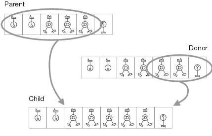
Figure 8.12: Recombination using transfer and remove. Note that the number of output terminal components in a program representation is fixed, so any that are transferred from the donor replace those copied from the parent.
Uniform crossover is a disruptive recombination operator which can be used to measure how program representations react both to high levels of change and to conventional evolutionary computation search operators. The second kind of recombination used by enzyme GP, termed transfer and remove, is used to observe how program representations react to lower levels of specific kinds of change. Transfer and remove recombination uses two complementary operators - transfer and remove - and takes advantage of the fact that components which are added to a program representation need not replace existing components. The transfer operator forms a child program representation by copying a contiguous sequence of components from one program representation (the donor) to another (the parent) without removing any existing components (with the exception of output terminals, whose numbers remain constant - see figure 8.12). The remove operator forms a child program representation by removing a contiguous sequence of components from a parent program representation. Each of these operations is used, non-deterministically, for 50% of crossover events. The effect of the remove operation is to balance solution sizes so that recombination has an overall neutral effect upon solution size within a population. For both transfer and remove operations, the number of components targeted is chosen randomly within an upper limit.
This chapter has introduced a form of genetic programming based upon an implicit context program representation in which interactions between program components are specified via behavioural descriptions rather than by position or other arbitrary references. Implicit context representation is expected to lead to a process of meaningful variation filtering whereby inappropriate change induced by variation operators can be wholly or partially ignored as a consequence of program behaviours emerging from the self-organisation of program components - ignoring those components which do not fit the contexts declared by the other components within the program.